Chapter 6 TECATOR dataset

In this chapter, we will focus on the application of previously described methods (for more details, see, for example, section 1) to real data tecator, which are available, for example, in the ddalpha package. A detailed description of the data can be found here. This dataset contains spectrometric curves (absorbance curves measured at 100 wavelengths).

For each piece of finely chopped meat, we observe one spectrometric curve, which corresponds to the absorbance measured at 100 wavelengths. The pieces are divided, according to Ferraty and Vieu (2006), into two classes: with low (\(< 20\%\)) and high (\(\geq 20\%\)) fat content obtained through analytical chemical processing. Our goal will be to classify the spectrometric curves on the interval \(I = [850 \text{ nm}, 1050 \text{ nm}]\) based on fat content. As we will see from the results in section 6.4, it is advantageous to consider the second derivative of the curves.

Let’s start by loading and plotting the data. The data are stored in a somewhat complex way, so to make working with them easier, we will save them in a more practical format. We will also name the respective columns according to whether the fat content is low (small) or high (large).

Code

# loading data 
library(fda)
library(ggplot2)
library(dplyr)
library(tidyr)
library(ddalpha)

data <- ddalpha::dataf.tecator()

data.gr <- data$dataf[[1]]$vals
for(i in 2:length(data$labels)) {
  data.gr <- rbind(data.gr, data$dataf[[i]]$vals)
  }
data.gr <- cbind(data.frame(wave = data$dataf[[1]]$args),
                 t(data.gr))

# vector of classes
labels <- data$labels |> unlist()
# renaming according to class
colnames(data.gr) <- c('wavelength',
                       paste0(labels, 1:length(data$labels)))

Let’s plot the spectrometric curves by group.

Code

abs.labs <- c("Fat content < 20 %", "Fat content > 20 %")
names(abs.labs) <- c('small', 'large')

pivot_longer(data.gr, cols = large1:large215, names_to = 'sample',
                        values_to = 'absorbance', cols_vary = 'slowest') |>
  mutate(sample = as.factor(sample),
         Abs = factor(rep(labels, each = length(data.gr$wavelength)), 
                      levels = c('small', 'large'))) |>
  ggplot(aes(x = wavelength, y = absorbance, colour = Abs, group = sample)) + 
  geom_line(linewidth = 0.5) + 
  theme_bw() +
  facet_wrap(~Abs,
             labeller = labeller(Abs = abs.labs)) + 
  labs(x = "Wavelength [in nm]",
       y = "Absorbance",
       colour = "Fat content") + 
  theme(legend.position = 'none') +
  scale_color_discrete(labels = abs.labs)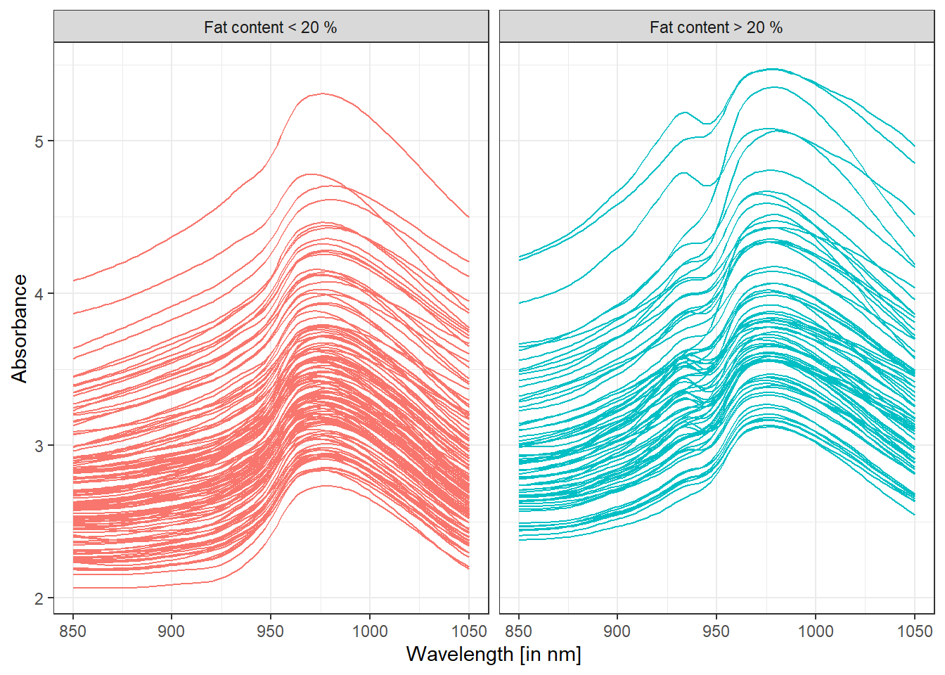

Figure 6.1: Absorbance curves by group.

6.1 Smoothing of Observed Curves

We will now transform the observed discrete values (value vectors) into functional objects, with which we will subsequently work. Since these are non-periodic curves on the interval \(I = [850, 1050]\), we will use a B-spline basis for smoothing.

We take the entire wavelength vector as knots, and we would normally consider cubic splines, but since we want to work with the second derivative, we choose norder = 6. For the same reason, we will penalize the fourth derivative of the functions.

Code

t <- data.gr$wavelength
rangeval <- range(t)
breaks <- t
norder <- 6

bbasis <- create.bspline.basis(rangeval = rangeval, 
                               norder = norder, 
                               breaks = breaks)

curv.Lfd <- int2Lfd(4) # penalize 4th derivative

We will find a suitable value of the smoothing parameter \(\lambda > 0\) using \(GCV(\lambda)\), i.e., generalized cross-validation. The value of \(\lambda\) will be considered the same for both classes, as for test observations we would not know in advance which value of \(\lambda\) to choose if different values were selected for each class.

Code

# combine observations into one matrix
XX <- data.gr[, -1] |> as.matrix()

lambda.vect <- 10^seq(from = -1, to = 0.5, length.out = 50) # lambda vector
gcv <- rep(NA, length = length(lambda.vect)) # empty vector for GCV storage

for(index in 1:length(lambda.vect)) {
  curv.Fdpar <- fdPar(bbasis, curv.Lfd, lambda.vect[index])
  BSmooth <- smooth.basis(t, XX, curv.Fdpar) # smoothing
  gcv[index] <- mean(BSmooth$gcv) # average across all observed curves
}

GCV <- data.frame(
  lambda = round(log10(lambda.vect), 3),
  GCV = gcv
)

# find the minimum value
lambda.opt <- lambda.vect[which.min(gcv)]

To illustrate better, we will plot the \(GCV(\lambda)\) progression.

Code

GCV |> ggplot(aes(x = lambda, y = GCV)) + 
  geom_line(linetype = 'solid', linewidth = 0.6) + 
  geom_point(size = 1.7) + 
  theme_bw() + 
  labs(x = bquote(paste(log[10](lambda), ' ;   ', 
                        lambda[optimal] == .(round(lambda.opt, 4)))),
       y = expression(GCV(lambda))) + 
  geom_point(aes(x = log10(lambda.opt), y = min(gcv)), colour = 'red', size = 3)

## Warning in geom_point(aes(x = log10(lambda.opt), y = min(gcv)), colour = "red", : All aesthetics have length 1, but the data has 50 rows.
## ℹ Please consider using `annotate()` or provide this layer with data containing
##   a single row.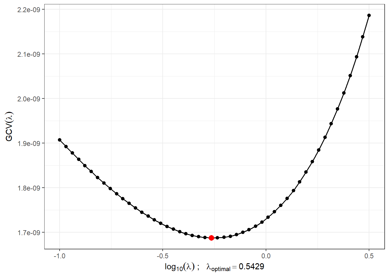

Figure 6.2: Progression of \(GCV(\lambda)\) for the chosen \(\boldsymbol\lambda\) vector. On the \(x\)-axis, values are shown on a logarithmic scale with base 10. The optimal value of the smoothing parameter \(\lambda_{optimal}\) is marked in red.

With this optimal choice of the smoothing parameter \(\lambda\), we will now smooth all functions.

Code

curv.fdPar <- fdPar(bbasis, curv.Lfd, lambda.opt)
BSmooth <- smooth.basis(t, XX, curv.fdPar)
XXfd <- BSmooth$fd

fdobjSmootheval <- eval.fd(fdobj = XXfd, evalarg = t)

Finally, we will display all curves including the average separately for each class.

Code

library(tikzDevice)
n <- dim(XX)[2]

DFsmooth <- data.frame(
  t = rep(t, n),
  time = factor(rep(1:n, each = length(t))),
  Smooth = c(fdobjSmootheval),
  Fat = factor(rep(labels, each = length(t)), levels = c('small', 'large'))
)

DFmean <- data.frame(
  t = rep(t, 2),
  Mean = c(eval.fd(fdobj = mean.fd(XXfd[labels == 'small']), evalarg = t),
           eval.fd(fdobj = mean.fd(XXfd[labels == 'large']), evalarg = t)),
  # c(apply(fdobjSmootheval[ , labels == 'small'], 1, mean), 
  #           apply(fdobjSmootheval[ , labels == 'large'], 1, mean)),
  Fat = factor(rep(c('small', 'large'), each = length(t)),
                 levels = c('small', 'large'))
)

DFsmooth |> ggplot(aes(x = t, y = Smooth, color = Fat)) + 
  geom_line(linewidth = 0.05, aes(group = time), alpha = 0.5) +
  theme_bw() +
  facet_wrap(~Fat,
             labeller = labeller(Fat = abs.labs)
             ) + 
  labs(x = "Wavelength",
       y = "Absorbance",
       colour = "Fat content") + 
  theme(legend.position = 'none') +
  geom_line(data = DFmean, aes(x = t, y = Mean), 
            colour = 'grey2', linewidth = 1.25, linetype = 'solid') +
  scale_colour_manual(values = c('tomato', 'deepskyblue2'))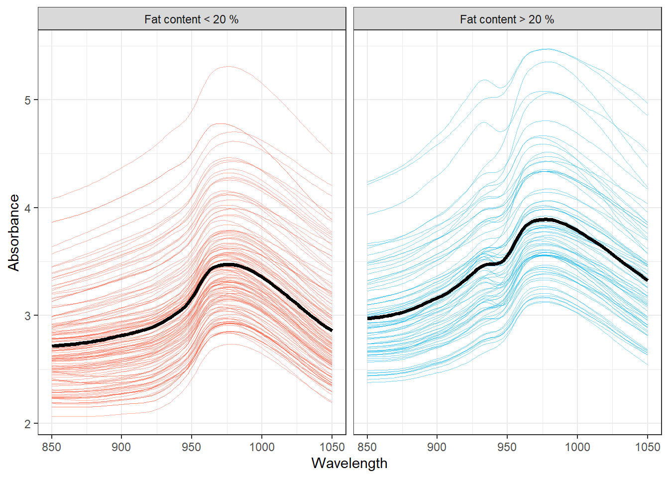

Figure 6.3: Plot of all smoothed observed curves, with colors distinguishing curves by class. The average for each class is shown in black.

Code

# ggsave("figures/kap7_tecator_curves_mean.tex", device = tikz, width = 9, height = 4.5)

We observe that the curves for both groups (by fat content) are relatively similar, with the average indicated in black. The curves differ mainly in the middle of the interval, where fattier samples show one additional local extremum, while less fatty samples appear simpler with only one extremum.

6.2 Computation of Derivatives

As mentioned above, it will be advantageous to classify the curves based on the second derivative. To compute the derivative for a functional object, we will use the deriv.fd() function from the fda package in R. Since we want to classify based on the second derivative, we set the argument Lfdobj = 2. The use of this data will be shown in Section 6.4.

Code

XXder <- deriv.fd(XXfd, 2)
ttt <- seq(min(t), max(t), length = 501)
fdobjSmootheval_der2 <- eval.fd(fdobj = XXder, 
                                evalarg = ttt)

Let’s display all curves, including the average, separately for each class.

Code

DFsmooth <- data.frame(
  t = rep(ttt, n),
  time = factor(rep(1:n, each = length(ttt))),
  Smooth = c(fdobjSmootheval_der2),
  Fat = factor(rep(labels, each = length(ttt)), levels = c('small', 'large'))
)

DFmean <- data.frame(
  t = rep(ttt, 2),
  Mean = c(eval.fd(fdobj = mean.fd(XXder[labels == 'small']), evalarg = ttt),
           eval.fd(fdobj = mean.fd(XXder[labels == 'large']), evalarg = ttt)),
  Fat = factor(rep(c('small', 'large'), each = length(ttt)),
                 levels = c('small', 'large'))
)

DFsmooth |> ggplot(aes(x = t, y = Smooth, color = Fat)) + 
  geom_line(linewidth = 0.05, aes(group = time), alpha = 0.5) +
  theme_bw() +
  facet_wrap(~Fat) + 
  labs(x = "Wavelength",
       y = "Absorbance",
       colour = "Fat content") + 
  theme(legend.position = 'none') +
  geom_line(data = DFmean, aes(x = t, y = Mean), 
            colour = 'grey2', linewidth = 1.25, linetype = 'solid') +
  scale_colour_manual(values = c('tomato', 'deepskyblue2'))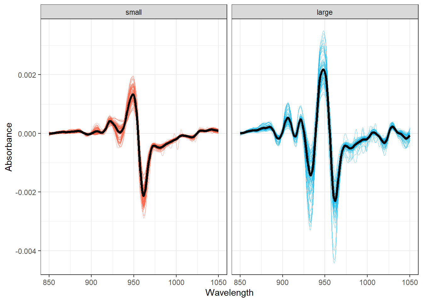

Figure 6.4: Plot of all smoothed observed curves, with colors distinguishing curves by classification class. The average for each class is shown in black.

Code

# ggsave("figures/kap7_tecator_curves_derivatives.tex", device = tikz, width = 9, height = 4.5)

From the figure above, we see that the average curves between the two groups of samples now differ much more significantly than in the case of the original non-derivative curves.

6.3 Classification of Original Curves

In the first part of this chapter, we will focus on the classification of the original non-derivative curves. Classification based on the second derivative of the original curves will be shown later in Section 6.4. First, we will load the necessary libraries for classification.

Code

library(caTools) # for splitting into test and training
library(caret) # for k-fold CV
library(fda.usc) # for KNN, fLR
library(MASS) # for LDA
library(fdapace)
library(pracma)
library(refund) # for LR on scores
library(nnet) # for LR on scores
library(caret)
library(rpart) # trees
library(rattle) # graphics
library(e1071)
library(randomForest) # random forest

set.seed(42)

We will split the data in a 30:70 ratio into test and training sets to evaluate the classification accuracy of individual methods. The training set will be used to construct the classifier, while the test set will be used to calculate the classification error and potentially other characteristics of our model. The resulting classifiers can then be compared with each other in terms of their classification accuracy based on these calculated characteristics.

Code

# splitting into test and training set
set.seed(42)
split <- sample.split(XXfd$fdnames$reps, SplitRatio = 0.7)

# creating a 0 and 1 vector, 0 for < 20 and 1 for > 20 
Y <- ifelse(labels == 'large', 1, 0)

X.train <- subset(XXfd, split == TRUE)
X.test <- subset(XXfd, split == FALSE)

Y.train <- subset(Y, split == TRUE)
Y.test <- subset(Y, split == FALSE)

Let’s check the distribution of individual groups in the test and training parts of the data.

Code

# absolute distribution
table(Y.train)

## Y.train
##  0  1 
## 91 59

Code

table(Y.test)

## Y.test
##  0  1 
## 47 18

Code

# relative distribution
table(Y.train) / sum(table(Y.train))

## Y.train
##         0         1 
## 0.6066667 0.3933333

Code

table(Y.test) / sum(table(Y.test))

## Y.test
##         0         1 
## 0.7230769 0.2769231

6.3.1 \(K\) Nearest Neighbors

We start with a non-parametric classification method, specifically the \(K\) nearest neighbors method. First, we create the necessary objects to work with the classif.knn() function from the fda.usc package.

Code

x.train <- fdata(X.train)
y.train <- as.numeric(factor(Y.train))

Now, we can define the model and examine its classification accuracy. The remaining question is how to choose the optimal number of neighbors \(K\). We could choose this \(K\) value as the one that minimizes the error on the training data. However, this might lead to overfitting, so we will use cross-validation. Given the computational complexity and size of the dataset, we choose \(k\)-fold CV, with \(k = 10\) for example.

Code

# model for all training data for K = 1, 2, ..., sqrt(n_train)
neighb.model <- classif.knn(group = y.train, 
                            fdataobj = x.train, 
                            knn = c(1:round(sqrt(length(y.train))))) 

1 - neighb.model$max.prob # minimum error

## [1] 0.1466667

Code

(K.opt <- neighb.model$h.opt) # optimal value of K

## [1] 1

Let’s apply this process to the training data, which we will split into \(k\) parts and repeat this code section \(k\) times.

Code

k_cv <- 10 # k-fold CV
neighbours <- c(1:(2 * ceiling(sqrt(length(y.train))))) # number of neighbors 

# split training data into k parts
folds <- createMultiFolds(X.train$fdnames$reps, k = k_cv, time = 1)

# empty matrix to store individual results
# columns will contain accuracy values for each training subset part
# rows will contain values for each K neighbors
CV.results <- matrix(NA, nrow = length(neighbours), ncol = k_cv)

for (index in 1:k_cv) {
  # define the index set
  fold <- folds[[index]]
    
  x.train.cv <- subset(X.train, c(1:length(X.train$fdnames$reps)) %in% fold) |>
    fdata()
  y.train.cv <- subset(Y.train, c(1:length(X.train$fdnames$reps)) %in% fold) |>
    factor() |> as.numeric()
  
  x.test.cv <- subset(X.train, !c(1:length(X.train$fdnames$reps)) %in% fold) |>
    fdata()
  y.test.cv <- subset(Y.train, !c(1:length(X.train$fdnames$reps)) %in% fold) |>
    factor() |> as.numeric()
  
  # repeat for each part ... k times
  for(neighbour in neighbours) {
    # model for a specific K choice
    neighb.model <- classif.knn(group = y.train.cv, 
                              fdataobj = x.train.cv, 
                              knn = neighbour) 
    # prediction on validation part
    model.neighb.predict <- predict(neighb.model, 
                                    new.fdataobj = x.test.cv)
    # accuracy on validation part
    accuracy <- table(y.test.cv, model.neighb.predict) |> 
      prop.table() |> diag() |> sum()
    
    # store accuracy at position for given K and fold
    CV.results[neighbour, index] <- accuracy
  }
}

# calculate average accuracy for each K across folds
CV.results <- apply(CV.results, 1, mean)
K.opt <- which.max(CV.results)
optimal.cv.accuracy <- max(CV.results)
CV.results <- data.frame(K = neighbours, CV = CV.results)

We see that the optimal value of the parameter \(K\) is 1, with an error rate calculated using 10-fold CV of 0.1478. For clarity, let’s plot the course of validation error with respect to the number of neighbors \(K\).

Code

CV.results |> ggplot(aes(x = K, y = 1 - CV)) + 
  geom_line(linetype = 'dashed', colour = 'grey') + 
  geom_point(size = 1.5) + 
  geom_point(aes(x = K.opt, y = 1 - optimal.cv.accuracy), colour = 'red', size = 2) +
  theme_bw() + 
  labs(x = bquote(paste(K, ' ;   ', 
                        K[optimal] == .(K.opt))),
       y = 'Validation Error') + 
  scale_x_continuous(breaks = neighbours)

## Warning in geom_point(aes(x = K.opt, y = 1 - optimal.cv.accuracy), colour = "red", : All aesthetics have length 1, but the data has 26 rows.
## ℹ Please consider using `annotate()` or provide this layer with data containing
##   a single row.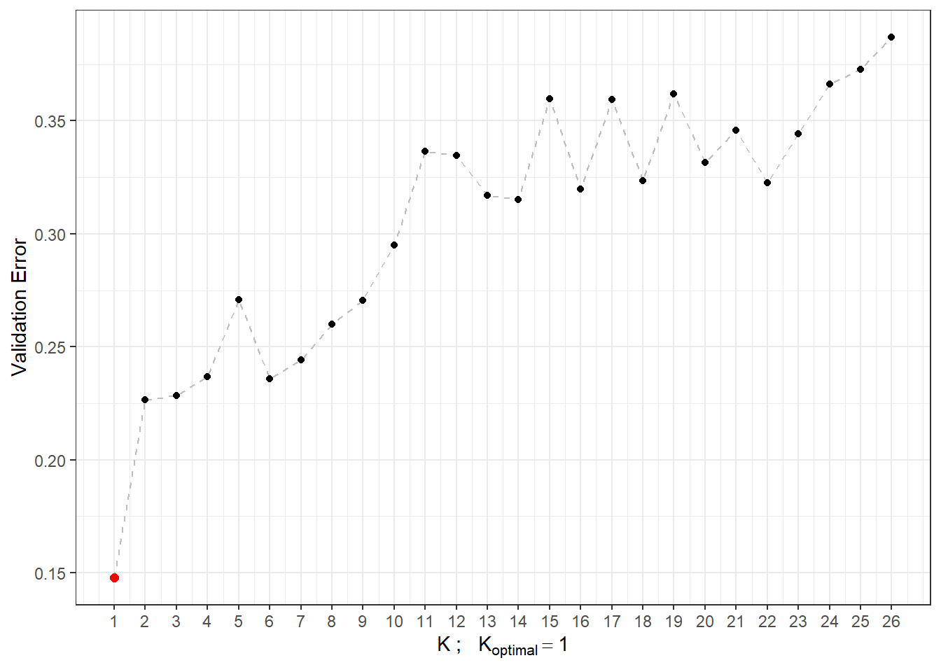

Figure 1.7: Dependence of validation error on the value of \(K\), i.e., on the number of neighbors.

Now that we know the optimal value of parameter \(K\), we can build the final model.

Code

neighb.model <- classif.knn(group = y.train, fdataobj = x.train, knn = K.opt)

# prediction
model.neighb.predict <- predict(neighb.model, 
                                new.fdataobj = fdata(X.test))

# accuracy on test data
accuracy <- table(as.numeric(factor(Y.test)), model.neighb.predict) |>
  prop.table() |>
  diag() |>
  sum()

Thus, we see that the error rate of the model built using the \(K\) nearest neighbors method with the optimal choice of \(K_{optimal}\) equal to 1, determined by cross-validation, is 0.1467 on the training data and 0.1692 on the test data.

To compare different models, we can use both types of error rates, and for clarity, we will store them in a table.

Code

RESULTS <- data.frame(model = 'KNN', 
                      Err.train = 1 - neighb.model$max.prob,
                      Err.test = 1 - accuracy)

6.3.2 Linear Discriminant Analysis

As a second method for constructing a classifier, we will consider linear discriminant analysis (LDA). Since this method cannot be applied to functional data directly, we first need to discretize the data, which we will do using functional principal component analysis. The classification algorithm will then be performed on the scores of the first \(p\) principal components. The number of components \(p\) is chosen so that the first \(p\) principal components together explain at least 90% of the variability in the data.

Let’s start by performing functional principal component analysis and determining the number \(p\).

Code

# principal component analysis
data.PCA <- pca.fd(X.train, nharm = 10) # nharm - maximum number of PCs
nharm <- which(cumsum(data.PCA$varprop) >= 0.9)[1] # determining p
if(nharm == 1) nharm <- 2 # to allow plotting graphs,
# we need at least 2 PCs

data.PCA <- pca.fd(X.train, nharm = nharm) 
data.PCA.train <- as.data.frame(data.PCA$scores) # scores of first p PCs
data.PCA.train$Y <- factor(Y.train) # class membership

In this specific case, we selected \(p=\) 2 as the number of principal components, which together explain 99.57 \(\%\) of the variability in the data. The first principal component explains 98.47 % and the second 1.09 \(\%\) of the variability. Graphically, we can display the scores of the first two principal components, with points colored according to class membership.

Code

data.PCA.train |> ggplot(aes(x = V1, y = V2, colour = Y)) +
  geom_point(size = 1.5) + 
  labs(x = paste('1st principal component (explained variability', 
                 round(100 * data.PCA$varprop[1], 2), '%)'),
       y = paste('2nd principal component (', 
                 round(100 * data.PCA$varprop[2], 2), '%)'),
       colour = 'Fat Content') +
  scale_color_discrete(labels = c("low", "high")) + 
  theme_bw()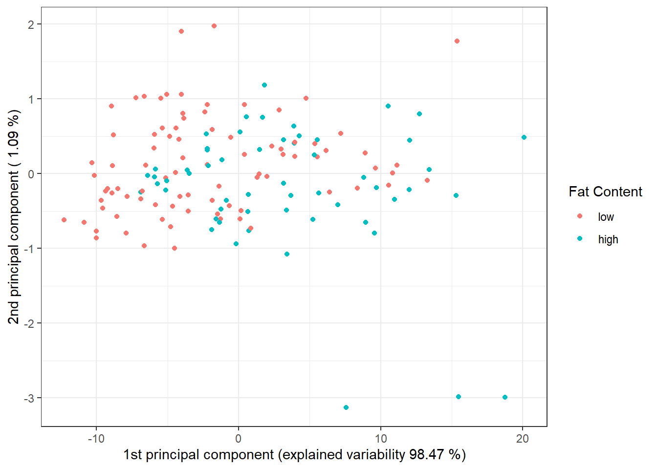

Figure 6.5: Scores of the first two principal components for the training data, with points colored by class membership.

To determine the classification accuracy on the test data, we need to calculate the scores for the first 2 principal components for the test data. These scores are calculated using the formula:

\[ \xi_{i, j} = \int \left( X_i(t) - \mu(t)\right) \cdot \rho_j(t) \, \text{dt}, \] where \(\mu(t)\) is the mean (average function) and \(\rho_j(t)\) are the eigenfunctions (functional principal components).

Code

# score calculation for test functions
scores <- matrix(NA, ncol = nharm, nrow = length(Y.test)) # empty matrix

for(k in 1:dim(scores)[1]) {
  xfd = X.test[k] - data.PCA$meanfd[1] # k-th observation - mean function
  scores[k, ] = inprod(xfd, data.PCA$harmonics) 
  # scalar product of residual and eigenfunctions rho (functional principal components)
}

data.PCA.test <- as.data.frame(scores)
data.PCA.test$Y <- factor(Y.test)
colnames(data.PCA.test) <- colnames(data.PCA.train) 

Now we can construct the classifier on the training data.

Code

# model
clf.LDA <- lda(Y ~ ., data = data.PCA.train)

# accuracy on training data
predictions.train <- predict(clf.LDA, newdata = data.PCA.train)
accuracy.train <- table(data.PCA.train$Y, predictions.train$class) |>
  prop.table() |> diag() |> sum()
  
# accuracy on test data
predictions.test <- predict(clf.LDA, newdata = data.PCA.test)
accuracy.test <- table(data.PCA.test$Y, predictions.test$class) |>
  prop.table() |> diag() |> sum()

We have calculated the error rate of the classifier on the training data (32 %) and on the test data (29.23 %).

For a graphical representation of the method, we can add the decision boundary to the plot of the scores of the first two principal components. This boundary is calculated on a dense grid of points and displayed using the geom_contour() function.

Code

# add discriminant boundary
np <- 1001 # number of grid points
# x-axis ... 1st PC
nd.x <- seq(from = min(data.PCA.train$V1), 
            to = max(data.PCA.train$V1), length.out = np)
# y-axis ... 2nd PC
nd.y <- seq(from = min(data.PCA.train$V2), 
            to = max(data.PCA.train$V2), length.out = np)
# case for 2 PCs ... p = 2
nd <- expand.grid(V1 = nd.x, V2 = nd.y)
# if p = 3
if(dim(data.PCA.train)[2] == 4) {
  nd <- expand.grid(V1 = nd.x, V2 = nd.y, V3 = data.PCA.train$V3[1])}
# if p = 4
if(dim(data.PCA.train)[2] == 5) {
  nd <- expand.grid(V1 = nd.x, V2 = nd.y, V3 = data.PCA.train$V3[1],
                    V4 = data.PCA.train$V4[1])}
# if p = 5
if(dim(data.PCA.train)[2] == 6) {
  nd <- expand.grid(V1 = nd.x, V2 = nd.y, V3 = data.PCA.train$V3[1],
                    V4 = data.PCA.train$V4[1], V5 = data.PCA.train$V5[1])}

# add Y = 0, 1
nd <- nd |> mutate(prd = as.numeric(predict(clf.LDA, newdata = nd)$class))

data.PCA.train |> ggplot(aes(x = V1, y = V2, colour = Y)) +
  geom_point(size = 1.5) + 
  labs(x = paste('1st principal component (explained variability', 
                 round(100 * data.PCA$varprop[1], 2), '%)'),
       y = paste('2nd principal component (', 
                 round(100 * data.PCA$varprop[2], 2), '%)'),
       colour = 'Fat Content') +
  scale_color_discrete(labels = c("low", "high")) + 
  theme_bw() +
  geom_contour(data = nd, aes(x = V1, y = V2, z = prd), colour = 'black')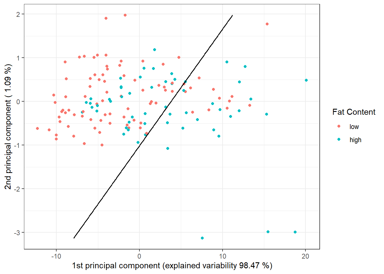

Figure 1.8: Scores of the first two principal components, colored by classification class. The black line represents the decision boundary (a line in the plane of the first two principal components) between classes constructed using LDA.

We observe that the decision boundary is a line, a linear function in the 2D space, as expected with LDA. Finally, we add the error rates to the summary table.

Code

Res <- data.frame(model = 'LDA', 
                  Err.train = 1 - accuracy.train,
                  Err.test = 1 - accuracy.test)

RESULTS <- rbind(RESULTS, Res)

6.3.3 Quadratic Discriminant Analysis

Next, let’s construct a classifier using Quadratic Discriminant Analysis (QDA). This approach is analogous to LDA, with the difference that we now allow for each class to have a distinct covariance matrix for the normal distribution from which the respective scores originate. This relaxed assumption of equal covariance matrices results in a quadratic boundary between classes.

In R, QDA is performed similarly to LDA as shown in the previous section; that is, we would calculate scores for both training and test functions using functional principal component analysis, construct a classifier on the scores of the first \(p\) principal components, and use it to predict the class membership of test curves in \(Y^* \in \{0, 1\}\).

We don’t need to perform functional PCA again, as we can use the results from the LDA section.

We can now proceed directly to constructing the classifier using the qda() function. We then calculate the classifier’s accuracy on the training and test data.

Code

# model
clf.QDA <- qda(Y ~ ., data = data.PCA.train)

# accuracy on training data
predictions.train <- predict(clf.QDA, newdata = data.PCA.train)
accuracy.train <- table(data.PCA.train$Y, predictions.train$class) |>
  prop.table() |> diag() |> sum()
  
# accuracy on test data
predictions.test <- predict(clf.QDA, newdata = data.PCA.test)
accuracy.test <- table(data.PCA.test$Y, predictions.test$class) |>
  prop.table() |> diag() |> sum()

We have calculated the error rate of the classifier on the training data (32 %) and on the test data (30.77 %).

For a graphical representation of the method, we can add the decision boundary to the plot of the scores of the first two principal components. This boundary is calculated on a dense grid of points and displayed using the geom_contour() function, as we did for LDA.

Code

nd <- nd |> mutate(prd = as.numeric(predict(clf.QDA, newdata = nd)$class))

data.PCA.train |> ggplot(aes(x = V1, y = V2, colour = Y)) +
  geom_point(size = 1.5) + 
  labs(x = paste('1st principal component (explained variability', 
                 round(100 * data.PCA$varprop[1], 2), '%)'),
       y = paste('2nd principal component (', 
                 round(100 * data.PCA$varprop[2], 2), '%)'),
       colour = 'Fat Content') +
  scale_color_discrete(labels = c("low", "high")) + 
  theme_bw() +
  geom_contour(data = nd, aes(x = V1, y = V2, z = prd), colour = 'black')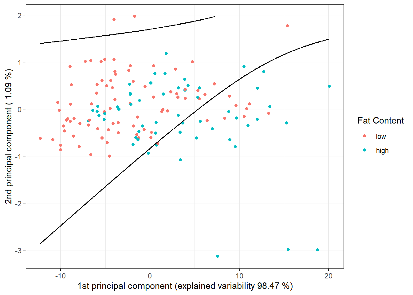

Figure 5.3: Scores of the first two principal components, colored by classification class. The black line represents the decision boundary (a parabola in the plane of the first two principal components) between classes constructed using QDA.

Notice that the decision boundary between the classification classes is now a parabola.

Finally, we add the error rates to the summary table.

Code

Res <- data.frame(model = 'QDA', 
                  Err.train = 1 - accuracy.train,
                  Err.test = 1 - accuracy.test)

RESULTS <- rbind(RESULTS, Res)

6.3.4 Logistic Regression

Logistic regression can be performed in two ways: either by using the functional equivalent of traditional logistic regression or by applying classical multivariate logistic regression on the scores of the first \(p\) principal components.

6.3.4.1 Functional Logistic Regression

Analogously to the finite-dimensional case, we consider a logistic model in the form:

\[ g\left(\mathbb E [Y|X = x]\right) = \eta (x) = g(\pi(x)) = \alpha + \int \beta(t)\cdot x(t) \text d t, \] where \(\eta(x)\) is the linear predictor with values in the interval \((-\infty, \infty)\), \(g(\cdot)\) is the link function (in the case of logistic regression, it is the logit function \(g: (0,1) \rightarrow \mathbb R,\ g(p) = \ln\frac{p}{1-p}\)), and \(\pi(x)\) is the conditional probability

\[ \pi(x) = \text{Pr}(Y = 1 | X = x) = g^{-1}(\eta(x)) = \frac{\text e^{\alpha + \int \beta(t)\cdot x(t) \text d t}}{1 + \text e^{\alpha + \int \beta(t)\cdot x(t) \text d t}}, \]

where \(\alpha\) is a constant, and \(\beta(t) \in L^2[a, b]\) is the parameter function. Our objective is to estimate this parameter function.

For functional logistic regression, we use the fregre.glm() function from the fda.usc package. First, we create appropriate objects for constructing the classifier.

Code

# Create appropriate objects
x.train <- fdata(X.train)
y.train <- as.numeric(Y.train) 

# Points where the functions are evaluated
tt <- x.train[["argvals"]]

dataf <- as.data.frame(y.train) 
colnames(dataf) <- "Y"

# Choose a basis for the functional observations, typically the same
# basis used for smoothing curves. However, this choice leads to numerical error,
# so we choose a basis with fewer functions. 
# After trying several options, 7 functions appear to be sufficient.
nbasis.x <- 100

# B-spline basis 
basis1 <- create.bspline.basis(rangeval = range(tt),
                               norder = 4,
                               nbasis = nbasis.x)

To estimate the parameter function \(\beta(t)\), we need to express it in a basis representation—in our case, a B-spline basis. However, we need to determine the appropriate number of basis functions. This could be decided based on the training error, but the training data will favor a larger number of bases, leading to model overfitting.

To illustrate this, let’s train a model on the training data for each basis count \(n_{basis} \in \{4, 5, \dots, 30\}\), calculate the training error, and also compute the test error. Note that to determine the optimal number of basis functions, we cannot use the same data as those for estimating the test error, as this would underestimate the error.

Code

n.basis.max <- 30
n.basis <- 4:n.basis.max
pred.baz <- matrix(NA, nrow = length(n.basis), ncol = 2, 
                   dimnames = list(n.basis, c('Err.train', 'Err.test')))

for (i in n.basis) {
  # Basis for beta
  basis2 <- create.bspline.basis(rangeval = range(tt), nbasis = i)
  # Relationship
  f <- Y ~ x
  # Basis for x and beta
  basis.x <- list("x" = basis1) # Smoothed data
  basis.b <- list("x" = basis2)
  # Model input data
  ldata <- list("df" = dataf, "x" = x.train)
  # Binomial model ... logistic regression model
  model.glm <- fregre.glm(f, family = binomial(), data = ldata,
                          basis.x = basis.x, basis.b = basis.b)
  
  # Accuracy on training data
  predictions.train <- predict(model.glm, newx = ldata)
  predictions.train <- data.frame(Y.pred = ifelse(predictions.train < 1/2, 0, 1))
  presnost.train <- table(Y.train, predictions.train$Y.pred) |>
    prop.table() |> diag() |> sum()
    
  # Accuracy on test data
  newldata = list("df" = as.data.frame(Y.test), "x" = fdata(X.test))
  predictions.test <- predict(model.glm, newx = newldata)
  predictions.test <- data.frame(Y.pred = ifelse(predictions.test < 1/2, 0, 1))
  presnost.test <- table(Y.test, predictions.test$Y.pred) |>
    prop.table() |> diag() |> sum()
  
  # Insert into matrix
  pred.baz[as.character(i), ] <- 1 - c(presnost.train, presnost.test)
} 

pred.baz <- as.data.frame(pred.baz)
pred.baz$n.basis <- n.basis

Let’s plot the dependence of both types of errors on the number of basis functions.

Code

n.basis.beta.opt <- pred.baz$n.basis[which.min(pred.baz$Err.test)]

pred.baz |> ggplot(aes(x = n.basis, y = Err.test)) + 
  geom_line(linetype = 'dashed', colour = 'black') + 
  geom_line(aes(x = n.basis, y = Err.train), colour = 'deepskyblue3', 
            linetype = 'dashed', linewidth = 0.5) + 
  geom_point(size = 1.5) + 
  geom_point(aes(x = n.basis, y = Err.train), colour = 'deepskyblue3', 
             size = 1.5) + 
  geom_point(aes(x = n.basis.beta.opt, y = min(pred.baz$Err.test)),
             colour = 'red', size = 2) +
  theme_bw() + 
  labs(x = bquote(paste(n[basis], ' ;   ', 
                        n[optimal] == .(n.basis.beta.opt))),
        y = 'Error')

## Warning: Use of `pred.baz$Err.test` is discouraged.
## ℹ Use `Err.test` instead.

## Warning in geom_point(aes(x = n.basis.beta.opt, y = min(pred.baz$Err.test)), : All aesthetics have length 1, but the data has 27 rows.
## ℹ Please consider using `annotate()` or provide this layer with data containing
##   a single row.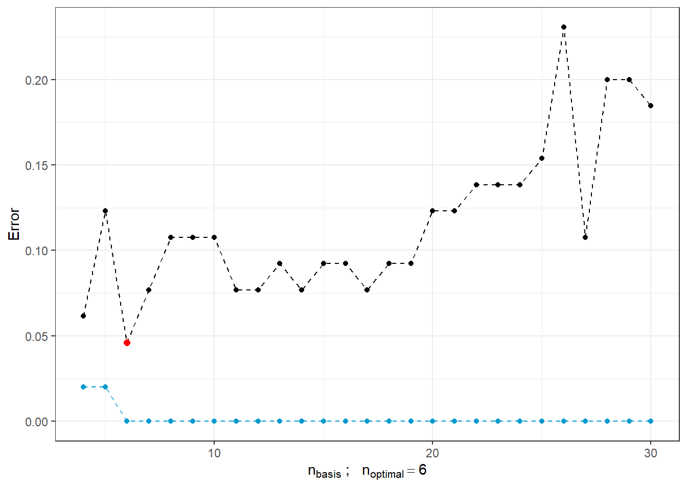

Figure 5.4: Dependence of test and training error on the number of basis functions for \(\beta\). The red dot represents the optimal number \(n_{optimal}\) chosen as the minimum test error, with the test error shown by the black line and training error by the blue dashed line.

We can see that with an increasing number of basis functions for \(\beta(t)\), the training error (blue line) tends to decrease, suggesting we would choose large values of \(n_{basis}\). However, the optimal choice based on the test error is \(n\) equal to 6, which is significantly smaller than 30. As \(n\) increases, the test error rises, indicating model overfitting.

To determine the optimal number of basis functions for \(\beta(t)\), we will use 10-fold cross-validation. The maximum number of considered basis functions is set to 25, as we observed earlier that values above this lead to overfitting.

Code

### 10-fold cross-validation
n.basis.max <- 25
n.basis <- 4:n.basis.max
k_cv <- 10 # k-fold CV
# divide training data into k parts
folds <- createMultiFolds(X.train$fdnames$reps, k = k_cv, time = 1)
## elements that remain unchanged during the cycle
# points where functions are evaluated
tt <- x.train[["argvals"]]
rangeval <- range(tt)
# B-spline basis 
# basis1 <- create.bspline.basis(rangeval = range(tt), nbasis = nbasis.x)
# relationship
f <- Y ~ x
# basis for x
basis.x <- list("x" = basis1)
# empty matrix to store individual results
# columns contain accuracy values for each part of the training set
# rows contain values for each basis count
CV.results <- matrix(NA, nrow = length(n.basis), ncol = k_cv, 
                     dimnames = list(n.basis, 1:k_cv))

Now we are ready to compute the error for each of the ten subsets of the training set. Next, we determine the average and take the argument of the minimum validation error as the optimal \(n\).

Code

for (index in 1:k_cv) {
  # define the index subset
  fold <- folds[[index]]
    
  x.train.cv <- subset(X.train, c(1:length(X.train$fdnames$reps)) %in% fold) |>
    fdata()
  y.train.cv <- subset(Y.train, c(1:length(X.train$fdnames$reps)) %in% fold) |>
    as.numeric()
  
  x.test.cv <- subset(X.train, !c(1:length(X.train$fdnames$reps)) %in% fold) |>
    fdata()
  y.test.cv <- subset(Y.train, !c(1:length(X.train$fdnames$reps)) %in% fold) |>
    as.numeric()
  
  dataf <- as.data.frame(y.train.cv) 
  colnames(dataf) <- "Y"
  
  for (i in n.basis) {
    # basis for betas
    basis2 <- create.bspline.basis(rangeval = rangeval, nbasis = i)
    
    basis.b <- list("x" = basis2)
    # input data for the model
    ldata <- list("df" = dataf, "x" = x.train.cv)
    # binomial model ... logistic regression model
    model.glm <- fregre.glm(f, family = binomial(), data = ldata,
                            basis.x = basis.x, basis.b = basis.b)
    
    # accuracy on the validation set 
    newldata = list("df" = as.data.frame(y.test.cv), "x" = x.test.cv)
    predictions.valid <- predict(model.glm, newx = newldata)
    predictions.valid <- data.frame(Y.pred = ifelse(predictions.valid < 1/2, 0, 1))
    presnost.valid <- table(y.test.cv, predictions.valid$Y.pred) |>
      prop.table() |> diag() |> sum()
    
    # insert into the matrix
    CV.results[as.character(i), as.character(index)] <- presnost.valid
  } 
}

# calculate average accuracy for each n across folds
CV.results <- apply(CV.results, 1, mean)
n.basis.opt <- n.basis[which.max(CV.results)]
presnost.opt.cv <- max(CV.results)

Let’s plot the course of validation error with the optimal value \(n_{optimal}\) marked, which is 19 with a validation error of 0.0604.

Code

CV.results <- data.frame(n.basis = n.basis, CV = CV.results)
CV.results |> ggplot(aes(x = n.basis, y = 1 - CV)) + 
  geom_line(linetype = 'dashed', colour = 'grey') + 
  geom_point(size = 1.5) + 
  geom_point(aes(x = n.basis.opt, y = 1 - presnost.opt.cv), colour = 'red', size = 2) +
  theme_bw() + 
  labs(x = bquote(paste(n[basis], ' ;   ', 
                        n[optimal] == .(n.basis.opt))),
       y = 'Validation error') + 
  scale_x_continuous(breaks = n.basis) + 
  theme(panel.grid.minor = element_blank())

## Warning in geom_point(aes(x = n.basis.opt, y = 1 - presnost.opt.cv), colour = "red", : All aesthetics have length 1, but the data has 22 rows.
## ℹ Please consider using `annotate()` or provide this layer with data containing
##   a single row.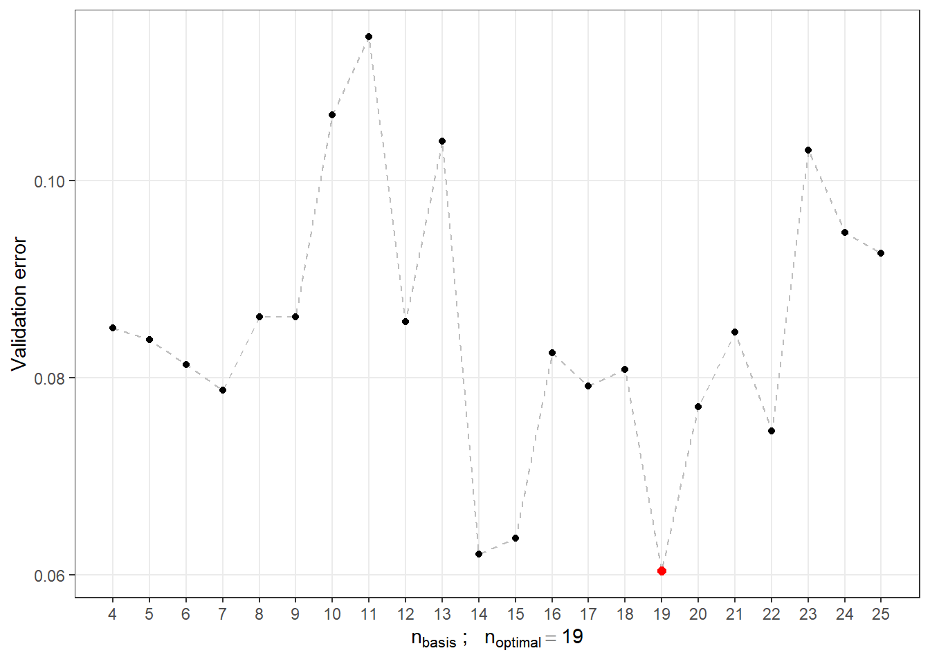

Figure 1.11: Dependence of validation error on the value of \(n_{basis}\), i.e., the number of bases.

We can now define the final model using functional logistic regression, choosing the B-spline basis for \(\beta(t)\) with 19 bases.

Code

# optimal model
basis2 <- create.bspline.basis(rangeval = range(tt), nbasis = n.basis.opt)
f <- Y ~ x
# basis for x and betas
basis.x <- list("x" = basis1) 
basis.b <- list("x" = basis2)
# input data for the model
dataf <- as.data.frame(y.train) 
colnames(dataf) <- "Y"
ldata <- list("df" = dataf, "x" = x.train)
# binomial model ... logistic regression model
model.glm <- fregre.glm(f, family = binomial(), data = ldata,
                        basis.x = basis.x, basis.b = basis.b,
                        maxit = 1000, epsilon = 1e-2)

# accuracy on the training data
predictions.train <- predict(model.glm, newx = ldata)
predictions.train <- data.frame(Y.pred = ifelse(predictions.train < 1/2, 0, 1))
presnost.train <- table(Y.train, predictions.train$Y.pred) |>
  prop.table() |> diag() |> sum()
  
# accuracy on the test data
newldata = list("df" = as.data.frame(Y.test), "x" = fdata(X.test))
predictions.test <- predict(model.glm, newx = newldata)
predictions.test <- data.frame(Y.pred = ifelse(predictions.test < 1/2, 0, 1))
presnost.test <- table(Y.test, predictions.test$Y.pred) |>
  prop.table() |> diag() |> sum()

We have calculated the training error (which is 0 %) and the test error (which is 9.23 %). To gain a better understanding, we can plot the estimated probabilities of belonging to the classification class \(Y = 1\) on the training data as a function of the linear predictor values.

Code

data.frame(
  linear.predictor = model.glm$linear.predictors,
  response = model.glm$fitted.values,
  Y = factor(y.train)
) |> ggplot(aes(x = linear.predictor, y = response, colour = Y)) + 
  geom_point(size = 1.5) + 
  scale_color_discrete(labels = c("small", "large")) + 
  geom_abline(aes(slope = 0, intercept = 0.5), linetype = 'dashed') + 
  theme_bw() + 
  labs(x = 'Linear Predictor',
       y = 'Estimated Probabilities Pr(Y = 1|X = x)',
       colour = 'Fat Content')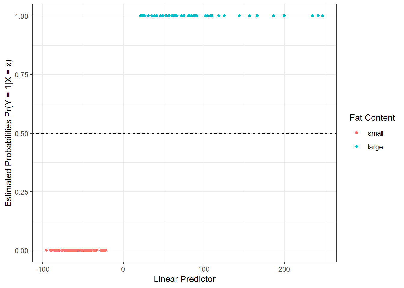 

Figure 6.6: Dependence of estimated probabilities on the values of the linear predictor. Points are colored based on their classification class.

Additionally, we can display the course of the estimated parametric function \(\beta(t)\) for reference.

Code

t.seq <- seq(min(t), max(t), length = 1001)
beta.seq <- eval.fd(evalarg = t.seq, fdobj = model.glm$beta.l$x)

data.frame(t = t.seq, beta = beta.seq) |>
  ggplot(aes(t, beta)) +
  geom_abline(aes(slope = 0, intercept = 0), linetype = 'dashed',
              linewidth = 0.5, colour = 'grey') +
  geom_line() +
  theme_bw() +
  labs(x = expression(x[1]),
       y = expression(widehat(beta)(t))) +
  theme(panel.grid.major = element_blank(),
        panel.grid.minor = element_blank())

Figure 4.1: Course of the estimated parametric function \(\beta(t), t \in [850, 1050]\).

Code

t.seq <- seq(min(tt), max(tt), length = 1001)
beta.seq <- eval.fd(evalarg = t.seq, fdobj = model.glm$beta.l$x)

# data.frame(t = t.seq, beta = beta.seq) |> 
#   ggplot(aes(t, beta)) + 
#   geom_abline(aes(slope = 0, intercept = 0), linetype = 'dashed', 
#               linewidth = 0.5, colour = 'grey') +
#   geom_line(colour = 'deepskyblue2', linewidth = 0.8) + 
#   theme_bw() +
#   labs(x = expression(t),
#        y = expression(widehat(beta)(t))) + 
#   theme(panel.grid.major = element_blank(),
#         panel.grid.minor = element_blank())
# 
# ggsave("figures/betahat_presentation.tex", width = 4, height = 2.5,
#        device = tikz)

Finally, we will add the results to the summary table.

Code

Res <- data.frame(model = 'LR functional', 
                  Err.train = 1 - presnost.train,
                  Err.test = 1 - presnost.test)

RESULTS <- rbind(RESULTS, Res)

6.3.4.2 Logistic Regression with Principal Component Analysis

To construct this classifier, we need to perform functional principal component analysis, determine the appropriate number of components, and calculate the score values for the test data. We have already done this in the linear discriminant analysis section, so we will utilize these results in the following part.

We can now directly build the logistic regression model using the glm(, family = binomial) function.

Code

# model
clf.LR <- glm(Y ~ ., data = data.PCA.train, family = binomial)

# accuracy on training data
predictions.train <- predict(clf.LR, newdata = data.PCA.train, type = 'response')
predictions.train <- ifelse(predictions.train > 0.5, 1, 0)
presnost.train <- table(data.PCA.train$Y, predictions.train) |>
  prop.table() |> diag() |> sum()

# accuracy on test data
predictions.test <- predict(clf.LR, newdata = data.PCA.test, type = 'response')
predictions.test <- ifelse(predictions.test > 0.5, 1, 0)
presnost.test <- table(data.PCA.test$Y, predictions.test) |>
  prop.table() |> diag() |> sum()

Thus, we have calculated the error rate of the classifier on the training data (30.67 %) and on the test data (29.23 %).

For graphical representation of the method, we can mark the decision boundary in the score plot of the first two principal components. We will calculate this boundary on a dense grid of points and display it using the geom_contour() function, as we did in the case of LDA and QDA.

Code

nd <- nd |> mutate(prd = as.numeric(predict(clf.LR, newdata = nd,
                                            type = 'response')))
nd$prd <- ifelse(nd$prd > 0.5, 1, 0)

data.PCA.train |> ggplot(aes(x = V1, y = V2, colour = Y)) +
  geom_point(size = 1.5) + 
  labs(x = paste('1st Principal Component (explained variability', 
                 round(100 * data.PCA$varprop[1], 2), '%)'),
       y = paste('2nd Principal Component (', 
                 round(100 * data.PCA$varprop[2], 2), '%)'),
       colour = 'Fat Content') +
  scale_colour_discrete(labels = c("small", "large")) +
  theme_bw() +
  geom_contour(data = nd, aes(x = V1, y = V2, z = prd), colour = 'black')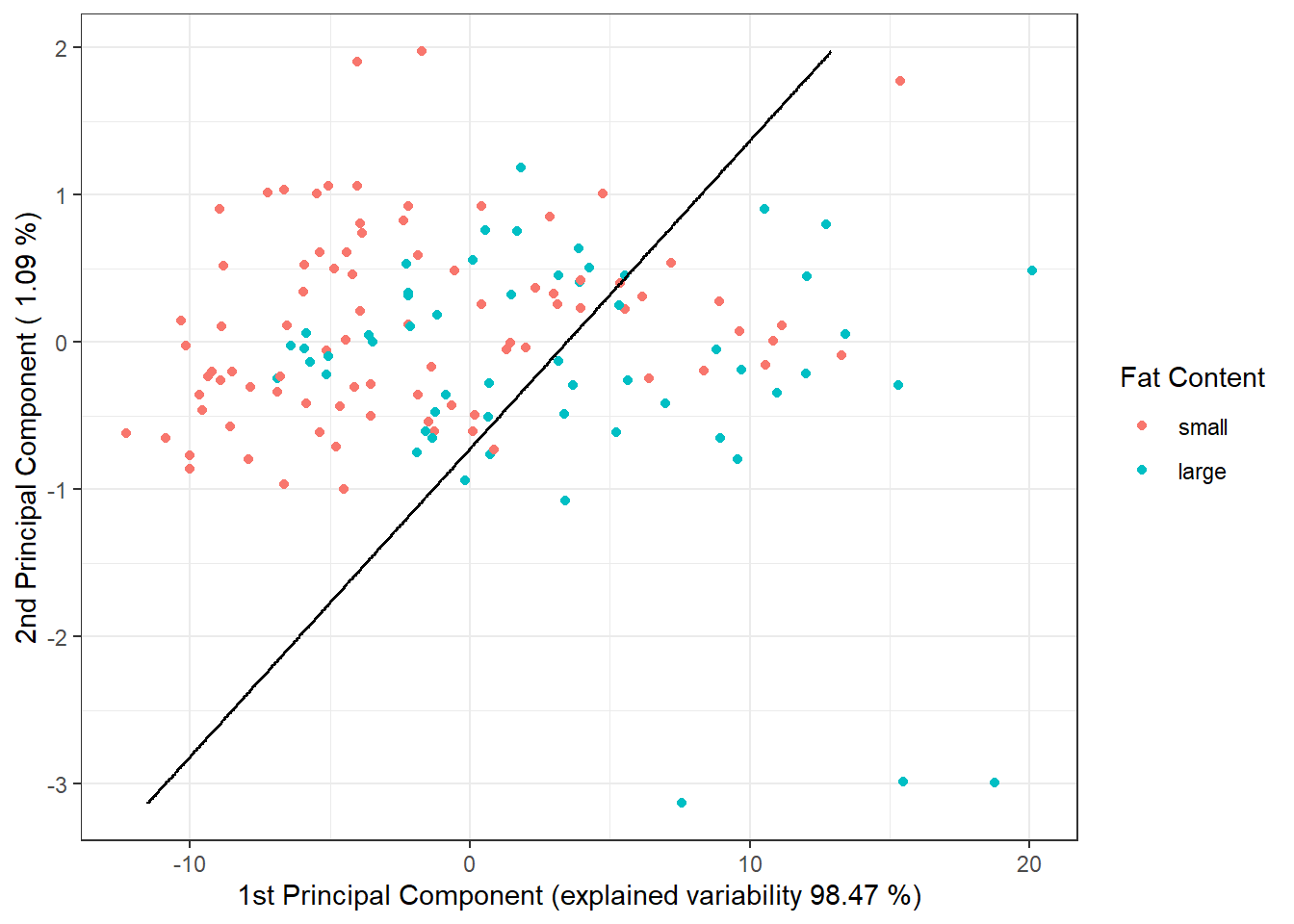

Figure 1.14: Scores of the first two principal components, colored according to class membership. The decision boundary (a line in the plane of the first two principal components) between classes, constructed using logistic regression, is marked in black.

Notice that the decision boundary between the classification classes is now a line, just like in the case of LDA.

Finally, we will add the error rates to the summary table.

Code

Res <- data.frame(model = 'LR score', 
                  Err.train = 1 - presnost.train,
                  Err.test = 1 - presnost.test)

RESULTS <- rbind(RESULTS, Res)

6.3.5 Decision Trees

In this section, we will explore a very different approach to constructing a classifier compared to methods like LDA or logistic regression. Decision trees are a popular tool for classification, but, similar to some previous methods, they are not directly designed for functional data. However, there are ways to transform functional objects into multidimensional data and then apply decision tree algorithms to them. We can consider the following approaches:

• An algorithm constructed on basis coefficients,
• Utilizing principal component scores,
• Discretizing the interval and evaluating the function only at a finite grid of points.

We will first focus on interval discretization and then compare the results with the other two approaches to constructing a decision tree.

6.3.5.1 Interval Discretization

First, we need to define the points from the interval \(I = [850, 1050]\), where we will evaluate the functions. Then we will create an object where the rows represent individual (discretized) functions and the columns represent time points. Finally, we will append a column \(Y\) containing information about class membership and repeat the same process for the test data.

Code

# sequence of points where we will evaluate the functions
t.seq <- seq(min(t), max(t), length = 101)
   
grid.data <- eval.fd(fdobj = X.train, evalarg = t.seq)
grid.data <- as.data.frame(t(grid.data)) # transpose to have functions in rows
grid.data$Y <- Y.train |> factor()

grid.data.test <- eval.fd(fdobj = X.test, evalarg = t.seq)
grid.data.test <- as.data.frame(t(grid.data.test))
grid.data.test$Y <- Y.test |> factor()

Now we can build a decision tree where all times from the t.seq vector will serve as predictors. This classification is not susceptible to multicollinearity, so we do not need to worry about it. We will choose accuracy as the metric.

Code

# building the model
clf.tree <- train(Y ~ ., data = grid.data, 
                 method = "rpart", 
                 trControl = trainControl(method = "CV", number = 10),
                 metric = "Accuracy")

# accuracy on training data
predictions.train <- predict(clf.tree, newdata = grid.data)
presnost.train <- table(Y.train, predictions.train) |>
  prop.table() |> diag() |> sum()
  
# accuracy on test data
predictions.test <- predict(clf.tree, newdata = grid.data.test)
presnost.test <- table(Y.test, predictions.test) |>
  prop.table() |> diag() |> sum()

The error rate of the classifier on the test data is thus 35.38 %, and on the training data, it is 29.33 %.

We can visualize the decision tree using the fancyRpartPlot() function. We will set the colors of the nodes to reflect the previous color distinctions. This is an unpruned tree.

Code

colnames(grid.data) <- c(paste0('time:', t.seq), 'Y')
fancyRpartPlot(rpart(Y ~ ., data = grid.data, method = "class"),
               sub = '', palettes = c('Reds', 'Blues')) 

Figure 5.6: Graphical representation of the unpruned decision tree. Nodes corresponding to class 1 are depicted in shades of blue, and those for class 0 in shades of red.

We can also plot the final pruned decision tree.

Code

rpart.plot::rpart.plot(clf.tree$finalModel, # final model ... pruned tree
                       extra = 104, # display desired information
                       box.palette = c('Reds', 'Blues'),
                       branch.lty = 3, # dotted branch lines
                       shadow.col = 0, # shadows under the node boxes
                       nn = FALSE, 
                       under = FALSE, 
                       digits = 2)

Figure 6.7: Final pruned decision tree.

Finally, we will again add the training and test error rates to the summary table.

Code

Res <- data.frame(model = 'Tree - discretization', 
                  Err.train = 1 - presnost.train,
                  Err.test = 1 - presnost.test)

RESULTS <- rbind(RESULTS, Res)

6.3.5.2 Principal Component Scores

Another option for constructing a decision tree is to use principal component scores. Since we have already calculated scores for previous classification methods, we will leverage this knowledge to build a decision tree based on the scores of the first 2 principal components.

Code

# building the model
clf.tree.PCA <- train(Y ~ ., data = data.PCA.train, 
                 method = "rpart", 
                 trControl = trainControl(method = "CV", number = 10),
                 metric = "Accuracy")

# accuracy on training data
predictions.train <- predict(clf.tree.PCA, newdata = data.PCA.train)
presnost.train <- table(Y.train, predictions.train) |>
  prop.table() |> diag() |> sum()
  
# accuracy on test data
predictions.test <- predict(clf.tree.PCA, newdata = data.PCA.test)
presnost.test <- table(Y.test, predictions.test) |>
  prop.table() |> diag() |> sum()

The error rate of the decision tree on the test data is thus 38.46 %, and on the training data, it is 32.67 %.

We can visualize the decision tree constructed from the principal component scores using the fancyRpartPlot() function. We will set the colors of the nodes to reflect the previous color distinctions. This is an unpruned tree.

Code

fancyRpartPlot(rpart(Y ~ ., data = data.PCA.train, method = "class"),
               sub = '', palettes = c('Reds', 'Blues')) 

Figure 5.7: Graphical representation of the unpruned decision tree constructed from principal component scores. Nodes corresponding to class 1 are depicted in shades of blue, and those for class 0 in shades of red.

We can also plot the final pruned decision tree.

Code

rpart.plot::rpart.plot(clf.tree.PCA$finalModel, # final model 
                       extra = 104, # display desired information
                       box.palette = c('Reds', 'Blues'),
                       branch.lty = 3, # dotted branch lines
                       shadow.col = 0, # shadows under the node boxes
                       nn = FALSE, under = FALSE, digits = 2)

Figure 6.8: Final pruned decision tree.

Finally, we will add the training and test error rates to the summary table.

Code

Res <- data.frame(model = 'Tree - score', 
                  Err.train = 1 - presnost.train,
                  Err.test = 1 - presnost.test)

RESULTS <- rbind(RESULTS, Res)

6.3.5.3 Basis Coefficients

The last option we will use to construct a decision tree is to utilize coefficients in the representation of functions in B-spline basis.

First, let’s define the necessary data files containing the coefficients.

Code

# training dataset
data.Bbasis.train <- t(X.train$coefs) |> as.data.frame()
data.Bbasis.train$Y <- factor(Y.train)

# testing dataset
data.Bbasis.test <- t(X.test$coefs) |> as.data.frame()
data.Bbasis.test$Y <- factor(Y.test)

Now we can build the classifier.

Code

# building the model
clf.tree.Bbasis <- train(Y ~ ., data = data.Bbasis.train, 
                 method = "rpart", 
                 trControl = trainControl(method = "CV", number = 10),
                 metric = "Accuracy")

# accuracy on training data
predictions.train <- predict(clf.tree.Bbasis, newdata = data.Bbasis.train)
presnost.train <- table(Y.train, predictions.train) |>
  prop.table() |> diag() |> sum()
  
# accuracy on test data
predictions.test <- predict(clf.tree.Bbasis, newdata = data.Bbasis.test)
presnost.test <- table(Y.test, predictions.test) |>
  prop.table() |> diag() |> sum()

The error rate of the decision tree on the training data is thus 22.67 %, and on the test data, it is 24.62 %.

We can visualize the decision tree constructed from the B-spline coefficients using the fancyRpartPlot() function. We will set the colors of the nodes to reflect the previous color distinctions. This is an unpruned tree.

Code

fancyRpartPlot(rpart(Y ~ ., data = data.Bbasis.train, method = "class"),
               sub = '', palettes = c('Reds', 'Blues')) 

Figure 5.8: Graphical representation of the unpruned decision tree constructed from basis coefficients. Nodes corresponding to class 1 are depicted in shades of blue, and those for class 0 in shades of red.

We can also plot the final pruned decision tree.

Code

rpart.plot::rpart.plot(clf.tree.Bbasis$finalModel, # final model 
                       extra = 104, # display desired information
                       box.palette = c('Reds', 'Blues'),
                       branch.lty = 3, # dotted branch lines
                       shadow.col = 0, # shadows under the node boxes
                       nn = FALSE, under = FALSE, digits = 2)

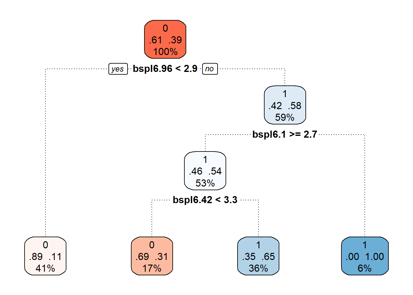
Figure 6.9: Final pruned decision tree.

Finally, we will add the training and test error rates to the summary table.

Code

Res <- data.frame(model = 'Tree - Bbasis', 
                  Err.train = 1 - presnost.train,
                  Err.test = 1 - presnost.test)

RESULTS <- rbind(RESULTS, Res)

6.3.6 Random Forests

A classifier constructed using the random forests method involves building several individual decision trees, which are then combined to create a common classifier through “voting.”

As with decision trees, we have several options regarding which data (finite-dimensional) we will use to construct the model. We will again consider the three approaches discussed earlier. The data files with the relevant variables for all three approaches have already been prepared in the previous section, so we can directly construct the models, calculate the characteristics of the classifier, and add the results to the summary table.

6.3.6.1 Interval Discretization

In the first case, we utilize the evaluation of functions at a grid of points in the interval \(I = [850, 1050]\).

Code

# building the model
clf.RF <- randomForest(Y ~ ., data = grid.data, 
                       ntree = 500, # number of trees
                       importance = TRUE,
                       nodesize = 5)

# accuracy on training data
predictions.train <- predict(clf.RF, newdata = grid.data)
presnost.train <- table(Y.train, predictions.train) |>
  prop.table() |> diag() |> sum()
  
# accuracy on test data
predictions.test <- predict(clf.RF, newdata = grid.data.test)
presnost.test <- table(Y.test, predictions.test) |>
  prop.table() |> diag() |> sum()

The error rate of the random forest on the training data is thus 2 %, and on the test data, it is 12.31 %.

Code

Res <- data.frame(model = 'RForest - discretization', 
                  Err.train = 1 - presnost.train,
                  Err.test = 1 - presnost.test)

RESULTS <- rbind(RESULTS, Res)

6.3.6.2 Principal Component Scores

In this case, we will use the scores of the first $p = $ 2 principal components.

Code

# building the model
clf.RF.PCA <- randomForest(Y ~ ., data = data.PCA.train, 
                           ntree = 500, # number of trees
                           importance = TRUE,
                           nodesize = 5)

# accuracy on training data
predictions.train <- predict(clf.RF.PCA, newdata = data.PCA.train)
presnost.train <- table(Y.train, predictions.train) |>
  prop.table() |> diag() |> sum()
  
# accuracy on test data
predictions.test <- predict(clf.RF.PCA, newdata = data.PCA.test)
presnost.test <- table(Y.test, predictions.test) |>
  prop.table() |> diag() |> sum()

The error rate of the random forest on the training data is thus 4.67 %, and on the test data, it is 30.77 %.

Code

Res <- data.frame(model = 'RForest - score', 
                  Err.train = 1 - presnost.train,
                  Err.test = 1 - presnost.test)

RESULTS <- rbind(RESULTS, Res)

6.3.6.3 Basis Coefficients

Finally, we will use the representation of functions through the B-spline basis.

Code

# building the model
clf.RF.Bbasis <- randomForest(Y ~ ., data = data.Bbasis.train, 
                              ntree = 500, # number of trees
                              importance = TRUE,
                              nodesize = 5)

# accuracy on training data
predictions.train <- predict(clf.RF.Bbasis, newdata = data.Bbasis.train)
presnost.train <- table(Y.train, predictions.train) |>
  prop.table() |> diag() |> sum()
  
# accuracy on test data
predictions.test <- predict(clf.RF.Bbasis, newdata = data.Bbasis.test)
presnost.test <- table(Y.test, predictions.test) |>
  prop.table() |> diag() |> sum()

The error rate of this classifier on the training data is 1.33 %, and on the test data, it is 12.31 %.

Code

Res <- data.frame(model = 'RForest - Bbasis', 
                  Err.train = 1 - presnost.train,
                  Err.test = 1 - presnost.test)

RESULTS <- rbind(RESULTS, Res)

6.3.7 Support Vector Machines

Now let’s take a look at curve classification using the Support Vector Machines (SVM) method. The advantage of this classification method is its computational efficiency, as it uses only a few (often very few) observations to define the decision boundary between classes.

The main advantage of SVM is the use of the so-called kernel trick, which allows us to replace the ordinary scalar product with another scalar product of transformed data, without having to explicitly define this transformation. This results in a generally nonlinear separating boundary between classification classes. A kernel (kernel function) \(K\) is a function that satisfies

\[ K(x_i, x_j) = \langle \phi(x_i), \phi(x_j) \rangle_{\mathcal H}, \] where \(\phi\) is some (unknown) transformation (feature map), \(\mathcal H\) is a Hilbert space, and \(\langle \cdot, \cdot \rangle_{\mathcal H}\) is some scalar product in this Hilbert space.

In practice, three types of kernel functions are most commonly chosen:

• Linear kernel – \(K(x_i, x_j) = \langle x_i, x_j \rangle\),
• Polynomial kernel – \(K(x_i, x_j) = \big(\alpha_0 + \gamma \langle x_i, x_j \rangle \big)^d\),
• Radial (Gaussian) kernel – \(\displaystyle{K(x_i, x_j) = \text e^{-\gamma \|x_i - x_j \|^2}}\).

For all the above-mentioned kernels, we must choose a constant \(C > 0\), which indicates the penalty for exceeding the decision boundary between classes (inverse regularization parameter). As the value of \(C\) increases, the method penalizes misclassified data more and the shape of the boundary less. Conversely, for small values of \(C\), the method does not give much importance to misclassified data but focuses more on penalizing the shape of the boundary. This constant \(C\) is typically set to 1 by default, but we can also determine it directly, for example, using cross-validation.

By utilizing cross-validation, we can also determine the optimal values of other hyperparameters, which now depend on our choice of kernel function. In the case of a linear kernel, no other parameters are chosen besides the constant \(C\). For polynomial and radial kernels, we must determine the hyperparameters \(\alpha_0, \gamma \text{ and } d\), whose default values in R are \(\alpha_0^{default} = 0, \gamma^{default} = \frac{1}{dim(\texttt{data})} \text{ and } d^{default} = 3\). We typically choose \(\alpha_0^{default} = 1\), as this value yields significantly better results.

When dealing with functional data, we have several options for applying the SVM method. The simplest variant is to use this classification method directly on the discretized function (section 6.3.7.2). Another option is to use the scores of the principal components and classify curves based on their representation (section 6.3.7.3). A straightforward variant is to use the representation of curves through the B-spline basis and classify curves based on the coefficients of their representation in this basis (section 6.3.7.4).

A more complex consideration leads us to several additional options that utilize the functional nature of the data. One option is to classify not the original curve but its derivative (or second, third derivatives, etc.). Another option is to utilize projections of functions onto a subspace generated, for example, by B-spline functions (section 6.3.7.5). The last method we will use for classifying functional data combines projection onto a certain subspace generated by functions (Reproducing Kernel Hilbert Space, RKHS) and classification of the corresponding representation. This method utilizes not only the classical SVM but also SVM for regression, which we elaborate on in section RKHS + SVM (section 6.3.7.6).

6.3.7.1 SVM for Functional Data

In the fda.usc library, we will use the function classif.svm() to apply the SVM method directly to functional data. First, we will create suitable objects for constructing the classifier.

Code

# set norm equal to one
norms <- c()
for (i in 1:dim(XXfd$coefs)[2]) {
  norms <- c(norms, as.numeric(1 / norm.fd(XXfd[i])))
}
XXfd_norm <- XXfd 
XXfd_norm$coefs <- XXfd_norm$coefs * matrix(norms, 
    ncol = dim(XXfd$coefs)[2],
    nrow = dim(XXfd$coefs)[1],
    byrow = T)

# splitting into test and training parts
X.train_norm <- subset(XXfd_norm, split == TRUE)
X.test_norm <- subset(XXfd_norm, split == FALSE)

Y.train_norm <- subset(Y, split == TRUE)
Y.test_norm <- subset(Y, split == FALSE)

Code

# create suitable objects
x.train <- fdata(X.train_norm)
y.train <- as.factor(Y.train_norm)

# points at which the functions are evaluated
tt <- x.train[["argvals"]]

dataf <- as.data.frame(y.train) 
colnames(dataf) <- "Y"
# B-spline basis 
nbasis.x <- 100
basis1 <- create.bspline.basis(rangeval = range(tt),
                               norder = 4,
                               nbasis = nbasis.x)

Code

# formula
f <- Y ~ x 
# basis for x
basis.x <- list("x" = basis1) 
# input data for the model
ldata <- list("df" = dataf, "x" = x.train)
# SVM model
model.svm.f <- classif.svm(formula = f,
            data = ldata,
            basis.x = basis.x,
            kernel = 'polynomial', degree = 3, coef0 = 1, cost = 1e4)

# accuracy on training data
newdat <- list("x" = x.train)
predictions.train <- predict(model.svm.f, newdat, type = 'class')
presnost.train <- mean(factor(Y.train_norm) == predictions.train)
  
# accuracy on test data
newdat <- list("x" = fdata(X.test_norm))
predictions.test <- predict(model.svm.f, newdat, type = 'class')
presnost.test <- mean(factor(Y.test_norm) == predictions.test)

We calculated the training error (which is 0 %) and the test error (which is 9.23 %).

Now let’s attempt, unlike the procedure in the previous chapters, to estimate the hyperparameters of the classifiers from the data using 10-fold cross-validation. Since each kernel has different hyperparameters in its definition, we will approach each kernel function separately. However, the hyperparameter \(C\) appears in all kernel functions, acknowledging that its optimal value may differ between kernels.

For all three kernels, we will explore the values of the hyperparameter \(C\) in the range \([10^{-2}, 10^{5}]\), while for the polynomial kernel, we will consider the value of the hyperparameter \(p\) to be 3, as other integer values do not yield nearly as good results. Conversely, for the radial kernel, we will again use \(r k_cv\)-fold CV to choose the optimal value of the hyperparameter \(\gamma\), considering values in the range \([10^{-5}, 10^{-2}]\). We will set coef0 to 1.

Code

set.seed(42)

k_cv <- 10 #  k-fold CV

# We split the training data into k parts
folds <- createMultiFolds(1:sum(split), k = k_cv, time = 1)

# Which values of gamma do we want to consider
gamma.cv <- 10^seq(-5, -2, length = 4)
C.cv <- 10^seq(-2, 5, length = 8)
p.cv <- 3
coef0 <- 1

# A list with three components... an array for each kernel -> linear, poly, radial
# An empty matrix where we will place individual results
# The columns will contain the accuracy values for each
# The rows will correspond to the values for a given gamma and the layers correspond to folds
CV.results <- list(
  SVM.l = array(NA, dim = c(length(C.cv), k_cv)),
  SVM.p = array(NA, dim = c(length(C.cv), length(p.cv), k_cv)),
  SVM.r = array(NA, dim = c(length(C.cv), length(gamma.cv), k_cv))
)

# First, we go through the values of C
for (cost in C.cv) {
  # We go through the individual folds
  for (index_cv in 1:k_cv) {
    # Definition of the test and training parts for CV
    fold <- folds[[index_cv]]
    cv_sample <- 1:dim(X.train_norm$coefs)[2] %in% fold
    
    x.train.cv <- fdata(subset(X.train_norm, cv_sample))
    x.test.cv <- fdata(subset(X.train_norm, !cv_sample))
    y.train.cv <- as.factor(subset(Y.train_norm, cv_sample))
    y.test.cv <- as.factor(subset(Y.train_norm, !cv_sample))
    
    # Points at which the functions are evaluated
    tt <- x.train.cv[["argvals"]]
    
    dataf <- as.data.frame(y.train.cv) 
    colnames(dataf) <- "Y"
    # B-spline basis
    # basis1 <- X.train_norm$basis
    # Formula
    f <- Y ~ x 
    # Basis for x
    basis.x <- list("x" = basis1) 
    # Input data for the model
    ldata <- list("df" = dataf, "x" = x.train.cv)
    
    ## LINEAR KERNEL
    # SVM model
    clf.svm.f_l <- classif.svm(formula = f,
                data = ldata,
                basis.x = basis.x,
                kernel = 'linear',
                cost = cost,
                type = 'C-classification',
                scale = TRUE)
      
    # Accuracy on the test data
    newdat <- list("x" = x.test.cv)
    predictions.test <- predict(clf.svm.f_l, newdat, type = 'class')
    accuracy.test.l <- mean(y.test.cv == predictions.test)
    
    # We insert the accuracies into positions for the given C and fold
    CV.results$SVM.l[(1:length(C.cv))[C.cv == cost], 
                     index_cv] <- accuracy.test.l
    
    ## POLYNOMIAL KERNEL
    for (p in p.cv) {
      # Model construction
      clf.svm.f_p <- classif.svm(formula = f,
                data = ldata,
                basis.x = basis.x,
                kernel = 'polynomial',
                cost = cost,
                coef0 = coef0,
                degree = p,
                type = 'C-classification',
                scale = TRUE)
        
      # Accuracy on the test data
      newdat <- list("x" = x.test.cv)
      predictions.test <- predict(clf.svm.f_p, newdat, type = 'class')
      accuracy.test.p <- mean(y.test.cv == predictions.test)
      
      # We insert the accuracies into positions for the given C, p, and fold
      CV.results$SVM.p[(1:length(C.cv))[C.cv == cost], 
                       (1:length(p.cv))[p.cv == p],
                       index_cv] <- accuracy.test.p
    }
        
    ## RADIAL KERNEL
    for (gam.cv in gamma.cv) {
      # Model construction
      clf.svm.f_r <- classif.svm(formula = f,
                data = ldata,
                basis.x = basis.x,
                kernel = 'radial',
                cost = cost,
                gamma = gam.cv,
                type = 'C-classification',
                scale = TRUE)
        
      # Accuracy on the test data
      newdat <- list("x" = x.test.cv)
      predictions.test <- predict(clf.svm.f_r, newdat, type = 'class')
      accuracy.test.r <- mean(y.test.cv == predictions.test)
      
      # We insert the accuracies into positions for the given C, gamma, and fold
      CV.results$SVM.r[(1:length(C.cv))[C.cv == cost], 
                       (1:length(gamma.cv))[gamma.cv == gam.cv],
                       index_cv] <- accuracy.test.r
    }
  }
}

Now we will average the results of 10-fold CV so that we have one estimate of validation error for one value of the hyperparameter (or one combination of values). At the same time, we will determine the optimal values of the individual hyperparameters.

Code

# We calculate the average accuracies for individual C across folds
## Linear kernel
CV.results$SVM.l <- apply(CV.results$SVM.l, 1, mean)
## Polynomial kernel
CV.results$SVM.p <- apply(CV.results$SVM.p, c(1, 2), mean)
## Radial kernel
CV.results$SVM.r <- apply(CV.results$SVM.r, c(1, 2), mean)

C.opt <- c(which.max(CV.results$SVM.l), 
           which.max(CV.results$SVM.p) %% length(C.cv), 
           which.max(CV.results$SVM.r) %% length(C.cv))
C.opt[C.opt == 0] <- length(C.cv)
C.opt <- C.cv[C.opt]

gamma.opt <- which.max(t(CV.results$SVM.r)) %% length(gamma.cv)
gamma.opt[gamma.opt == 0] <- length(gamma.cv)
gamma.opt <- gamma.cv[gamma.opt]

p.opt <- which.max(t(CV.results$SVM.p)) %% length(p.cv)
p.opt[p.opt == 0] <- length(p.cv)
p.opt <- p.cv[p.opt]

accuracy.opt.cv <- c(max(CV.results$SVM.l), 
                     max(CV.results$SVM.p),
                     max(CV.results$SVM.r))

Let’s take a look at how the optimal values turned out. For linear kernel, we have the optimal value \(C\) equal to 1, for polynomial kernel \(C\) is equal to 1, and for radial kernel, we have two optimal values, for \(C\) the optimal value is 10^{4} and for \(\gamma\) it is 0. The validation error rates are 0.0066667 for linear, 0.02625 for polynomial, and 0.0066667 for radial kernel.

Finally, we can construct the final classifiers on the entire training data with the hyperparameter values determined using 10-fold CV. We will also determine the errors on the test and training data.

Code

# Create suitable objects
x.train <- fdata(X.train_norm)
y.train <- as.factor(Y.train_norm)

# Points at which the functions are evaluated
tt <- x.train[["argvals"]]

dataf <- as.data.frame(y.train) 
colnames(dataf) <- "Y"
# B-spline basis
# basis1 <- X.train_norm$basis

# Formula
f <- Y ~ x 
# Basis for x
basis.x <- list("x" = basis1) 
# Input data for the model
ldata <- list("df" = dataf, "x" = x.train)

Code

model.svm.f_l <- classif.svm(formula = f,
            data = ldata,
            basis.x = basis.x,
            kernel = 'linear', 
            type = 'C-classification',
            scale = TRUE,
            cost = C.opt[1])

model.svm.f_p <- classif.svm(formula = f,
            data = ldata,
            basis.x = basis.x,
            kernel = 'polynomial', 
            type = 'C-classification',
            scale = TRUE,
            degree = p.opt,
            coef0 = coef0,
            cost = C.opt[2])

model.svm.f_r <- classif.svm(formula = f,
            data = ldata,
            basis.x = basis.x,
            kernel = 'radial', 
            type = 'C-classification',
            scale = TRUE,
            gamma = gamma.opt,
            cost = C.opt[3])

# Accuracy on training data
newdat <- list("x" = x.train)
predictions.train.l <- predict(model.svm.f_l, newdat, type = 'class')
accuracy.train.l <- mean(factor(Y.train_norm) == predictions.train.l)

predictions.train.p <- predict(model.svm.f_p, newdat, type = 'class')
accuracy.train.p <- mean(factor(Y.train_norm) == predictions.train.p)

predictions.train.r <- predict(model.svm.f_r, newdat, type = 'class')
accuracy.train.r <- mean(factor(Y.train_norm) == predictions.train.r)
  
# Accuracy on test data
newdat <- list("x" = fdata(X.test_norm))
predictions.test.l <- predict(model.svm.f_l, newdat, type = 'class')
accuracy.test.l <- mean(factor(Y.test_norm) == predictions.test.l)

predictions.test.p <- predict(model.svm.f_p, newdat, type = 'class')
accuracy.test.p <- mean(factor(Y.test_norm) == predictions.test.p)

predictions.test.r <- predict(model.svm.f_r, newdat, type = 'class')
accuracy.test.r <- mean(factor(Y.test_norm) == predictions.test.r)

The error rate of the SVM method on the training data is thus 0.6667 % for the linear kernel, 1.3333 % for the polynomial kernel, and 1.3333 % for the Gaussian kernel. On the test data, the error rate of the method is 9.2308 % for the linear kernel, 6.1538 % for the polynomial kernel, and 4.6154 % for the radial kernel.

Code

Res <- data.frame(model = c('SVM linear - func', 
                            'SVM poly - func', 
                            'SVM rbf - func'), 
                  Err.train = 1 - c(accuracy.train.l, accuracy.train.p, accuracy.train.r),
                  Err.test = 1 - c(accuracy.test.l, accuracy.test.p, accuracy.test.r))

RESULTS <- rbind(RESULTS, Res)

6.3.7.2 Discretization of the Interval

Let’s start by applying the Support Vector Machines method directly to the discretized data (evaluating the function on a given grid of points over the interval \(I = [850, 1050]\)), considering all three aforementioned kernel functions.

Code

# set norm equal to one
norms <- c()
for (i in 1:dim(XXfd$coefs)[2]) {
  norms <- c(norms, as.numeric(1 / norm.fd(BSmooth$fd[i])))
}
XXfd_norm <- XXfd 
XXfd_norm$coefs <- XXfd_norm$coefs * matrix(norms, 
                                            ncol = dim(XXfd$coefs)[2],
                                            nrow = dim(XXfd$coefs)[1],
                                            byrow = T)

# split into test and training sets
X.train_norm <- subset(XXfd_norm, split == TRUE)
X.test_norm <- subset(XXfd_norm, split == FALSE)

Y.train_norm <- subset(Y, split == TRUE)
Y.test_norm <- subset(Y, split == FALSE)

grid.data <- eval.fd(fdobj = X.train_norm, evalarg = t.seq)
grid.data <- as.data.frame(t(grid.data)) 
grid.data$Y <- Y.train_norm |> factor()

grid.data.test <- eval.fd(fdobj = X.test_norm, evalarg = t.seq)
grid.data.test <- as.data.frame(t(grid.data.test))
grid.data.test$Y <- Y.test_norm |> factor()

Now let’s estimate the hyperparameters of the classifiers from the data using 10-fold cross-validation. Since each kernel has different hyperparameters in its definition, we will approach each kernel function separately. However, the hyperparameter \(C\) appears in all kernel functions, and we allow for its optimal value to differ between kernels.

For all three kernels, we will explore values of the hyperparameter \(C\) in the interval \([10^{-3}, 10^{3}]\), fixing the hyperparameter \(p\) for the polynomial kernel at the value 3, since other integer values do not yield nearly as good results. For the radial kernel, we will again use 10-fold CV to choose the optimal value of the hyperparameter \(\gamma\), considering values in the interval \([10^{-4}, 10^{0}]\). We will set coef0 to \(= 1\).

Code

set.seed(42)

k_cv <- 10 # k-fold CV

# split training data into k parts
folds <- createMultiFolds(1:sum(split), k = k_cv, time = 1)

# values of gamma to consider
gamma.cv <- 10^seq(-4, 0, length = 5)
C.cv <- 10^seq(-3, 3, length = 7)
p.cv <- 3
coef0 <- 1

# list with three components ... array for individual kernels -> linear, poly, radial
# empty matrix to store results
# columns will contain accuracy values for given C
# rows will contain values for given gamma, and layers correspond to folds
CV.results <- list(
  SVM.l = array(NA, dim = c(length(C.cv), k_cv)),
  SVM.p = array(NA, dim = c(length(C.cv), length(p.cv), k_cv)),
  SVM.r = array(NA, dim = c(length(C.cv), length(gamma.cv), k_cv))
)

# first loop over values of C
for (C in C.cv) {
  # loop through the individual folds
  for (index_cv in 1:k_cv) {
    # define the test and training parts for CV
    fold <- folds[[index_cv]]
    cv_sample <- 1:dim(grid.data)[1] %in% fold
    
    data.grid.train.cv <- as.data.frame(grid.data[cv_sample, ])
    data.grid.test.cv <- as.data.frame(grid.data[!cv_sample, ])
    
    ## LINEAR KERNEL
    # model construction
    clf.SVM.l <- svm(Y ~ ., data = data.grid.train.cv,
                     type = 'C-classification',
                     scale = TRUE,
                     cost = C,
                     kernel = 'linear')
    
    # accuracy on validation data
    predictions.test.l <- predict(clf.SVM.l, newdata = data.grid.test.cv)
    accuracy.test.l <- table(data.grid.test.cv$Y, predictions.test.l) |>
      prop.table() |> diag() |> sum()
    
    # store accuracies for the respective C and fold
    CV.results$SVM.l[(1:length(C.cv))[C.cv == C], 
                     index_cv] <- accuracy.test.l
    
    ## POLYNOMIAL KERNEL
    for (p in p.cv) {
      # model construction
      clf.SVM.p <- svm(Y ~ ., data = data.grid.train.cv,
                       type = 'C-classification',
                       scale = TRUE,
                       cost = C,
                       coef0 = coef0,
                       degree = p,
                       kernel = 'polynomial')
      
      # accuracy on validation data
      predictions.test.p <- predict(clf.SVM.p, newdata = data.grid.test.cv)
      accuracy.test.p <- table(data.grid.test.cv$Y, predictions.test.p) |>
        prop.table() |> diag() |> sum()
      
      # store accuracies for the respective C, p, and fold
      CV.results$SVM.p[(1:length(C.cv))[C.cv == C], 
                       (1:length(p.cv))[p.cv == p],
                       index_cv] <- accuracy.test.p
    }
        
    ## RADIAL KERNEL
    for (gamma in gamma.cv) {
      # model construction
      clf.SVM.r <- svm(Y ~ ., data = data.grid.train.cv,
                       type = 'C-classification',
                       scale = TRUE,
                       cost = C,
                       gamma = gamma,
                       kernel = 'radial')
      
      # accuracy on validation data
      predictions.test.r <- predict(clf.SVM.r, newdata = data.grid.test.cv)
      accuracy.test.r <- table(data.grid.test.cv$Y, predictions.test.r) |>
        prop.table() |> diag() |> sum()
      
      # store accuracies for the respective C, gamma, and fold
      CV.results$SVM.r[(1:length(C.cv))[C.cv == C], 
                       (1:length(gamma.cv))[gamma.cv == gamma],
                       index_cv] <- accuracy.test.r
    }
  }
}

Now we average the results of the 10-fold cross-validation so that we have a single estimate of validation error for each value of the hyperparameter (or each combination of values). We will also determine the optimal values of the individual hyperparameters.

Code

# Calculate average accuracies for each C across folds
## Linear kernel
CV.results$SVM.l <- apply(CV.results$SVM.l, 1, mean)
## Polynomial kernel
CV.results$SVM.p <- apply(CV.results$SVM.p, c(1, 2), mean)
## Radial kernel
CV.results$SVM.r <- apply(CV.results$SVM.r, c(1, 2), mean)

C.opt <- c(which.max(CV.results$SVM.l), 
           which.max(CV.results$SVM.p) %% length(C.cv), 
           which.max(CV.results$SVM.r) %% length(C.cv))
C.opt[C.opt == 0] <- length(C.cv)
C.opt <- C.cv[C.opt]

gamma.opt <- which.max(t(CV.results$SVM.r)) %% length(gamma.cv)
gamma.opt[gamma.opt == 0] <- length(gamma.cv)
gamma.opt <- gamma.cv[gamma.opt]

p.opt <- which.max(t(CV.results$SVM.p)) %% length(p.cv)
p.opt[p.opt == 0] <- length(p.cv)
p.opt <- p.cv[p.opt]

presnost.opt.cv <- c(max(CV.results$SVM.l), 
                     max(CV.results$SVM.p),
                     max(CV.results$SVM.r))

Let’s look at the optimal values. For the linear kernel, we have an optimal value of \(C\) equal to 0.1; for the polynomial kernel, \(C\) is equal to 1; and for the radial kernel, we have two optimal values: the optimal value for \(C\) is 1000 and for \(\gamma\) it is 10^{-4}. The validation errors are 0.0066667 for linear, 0.0195833 for polynomial, and 0.0066667 for radial kernels.

Finally, we can construct the final classifiers on the entire training dataset using the hyperparameter values determined by the 10-fold cross-validation. We will also determine the errors on the test and training data.

Code

# Model construction
clf.SVM.l <- svm(Y ~ ., data = grid.data,
                 type = 'C-classification',
                 scale = TRUE,
                 cost = C.opt[1],
                 kernel = 'linear')

clf.SVM.p <- svm(Y ~ ., data = grid.data,
                 type = 'C-classification',
                 scale = TRUE,
                 cost = C.opt[2],
                 degree = p.opt,
                 coef0 = coef0,
                 kernel = 'polynomial')

clf.SVM.r <- svm(Y ~ ., data = grid.data,
                 type = 'C-classification',
                 scale = TRUE, 
                 cost = C.opt[3],
                 gamma = gamma.opt,
                 kernel = 'radial')

# Accuracy on training data
predictions.train.l <- predict(clf.SVM.l, newdata = grid.data)
presnost.train.l <- table(Y.train, predictions.train.l) |>
  prop.table() |> diag() |> sum()

predictions.train.p <- predict(clf.SVM.p, newdata = grid.data)
presnost.train.p <- table(Y.train, predictions.train.p) |>
  prop.table() |> diag() |> sum()

predictions.train.r <- predict(clf.SVM.r, newdata = grid.data)
presnost.train.r <- table(Y.train, predictions.train.r) |>
  prop.table() |> diag() |> sum()

# Accuracy on test data
predictions.test.l <- predict(clf.SVM.l, newdata = grid.data.test)
presnost.test.l <- table(Y.test, predictions.test.l) |>
  prop.table() |> diag() |> sum()

predictions.test.p <- predict(clf.SVM.p, newdata = grid.data.test)
presnost.test.p <- table(Y.test, predictions.test.p) |>
  prop.table() |> diag() |> sum()

predictions.test.r <- predict(clf.SVM.r, newdata = grid.data.test)
presnost.test.r <- table(Y.test, predictions.test.r) |>
  prop.table() |> diag() |> sum()

The error rate of the SVM method on the training data is therefore 1.3333 % for the linear kernel, 1.3333 % for the polynomial kernel, and 0.6667 % for the radial kernel. On the test data, the error rate of the method is 4.6154 % for the linear kernel, 4.6154 % for the polynomial kernel, and 9.2308 % for the radial kernel.

Code

Res <- data.frame(model = c('SVM linear - class', 
                            'SVM poly - class', 
                            'SVM rbf - class'), 
                  Err.train = 1 - c(presnost.train.l, presnost.train.p, presnost.train.r),
                  Err.test = 1 - c(presnost.test.l, presnost.test.p, presnost.test.r))

RESULTS <- rbind(RESULTS, Res)

6.3.7.3 Principal Component Scores

In this case, we will use the scores of the first $p = $ 2 principal components.

Now, let’s attempt to estimate the hyperparameters of the classifiers from the data using 10-fold cross-validation, differing from the approach in previous chapters. Since each kernel has different hyperparameters in its definition, we will approach each kernel function separately. However, the hyperparameter \(C\) is present in all kernel functions, allowing for the possibility that its optimal value may differ across kernels.

For all three kernels, we will examine values of the hyperparameter \(C\) in the interval \([10^{-3}, 10^{3}]\), while for the polynomial kernel we will fix the hyperparameter \(p\) at the value 3, as other integer values do not yield nearly as good results. Conversely, for the radial kernel, we will again use 10-fold cross-validation to choose the optimal value of the hyperparameter \(\gamma\), considering values in the interval \([10^{-3}, 10^{2}]\). We will set coef0 to \(= 1\).

Code

set.seed(42)

# Define the gamma values to consider
gamma.cv <- 10^seq(-3, 2, length = 6)
C.cv <- 10^seq(-3, 3, length = 7)
p.cv <- 3
coef0 <- 1

# List with three components... array for individual kernels -> linear, poly, radial
# Empty matrix to store results
# Columns will represent accuracies for given C values
# Rows will represent values for given gamma, with layers corresponding to folds
CV.results <- list(
  SVM.l = array(NA, dim = c(length(C.cv), k_cv)),
  SVM.p = array(NA, dim = c(length(C.cv), length(p.cv), k_cv)),
  SVM.r = array(NA, dim = c(length(C.cv), length(gamma.cv), k_cv))
)

# First, iterate over the values of C
for (C in C.cv) {
  # Iterate over the individual folds
  for (index_cv in 1:k_cv) {
    # Define the test and training parts for CV
    fold <- folds[[index_cv]]
    cv_sample <- 1:dim(data.PCA.train)[1] %in% fold
    
    data.PCA.train.cv <- as.data.frame(data.PCA.train[cv_sample, ])
    data.PCA.test.cv <- as.data.frame(data.PCA.train[!cv_sample, ])
    
    ## LINEAR KERNEL
    # Model construction
    clf.SVM.l <- svm(Y ~ ., data = data.PCA.train.cv,
                     type = 'C-classification',
                     scale = TRUE,
                     cost = C,
                     kernel = 'linear')
    
    # Accuracy on validation data
    predictions.test.l <- predict(clf.SVM.l, newdata = data.PCA.test.cv)
    presnost.test.l <- table(data.PCA.test.cv$Y, predictions.test.l) |>
      prop.table() |> diag() |> sum()
    
    # Store accuracies at positions for given C and fold
    CV.results$SVM.l[(1:length(C.cv))[C.cv == C], 
                     index_cv] <- presnost.test.l
    
    ## POLYNOMIAL KERNEL
    for (p in p.cv) {
      # Model construction
      clf.SVM.p <- svm(Y ~ ., data = data.PCA.train.cv,
                       type = 'C-classification',
                       scale = TRUE,
                       cost = C,
                       coef0 = coef0,
                       degree = p,
                       kernel = 'polynomial')
      
      # Accuracy on validation data
      predictions.test.p <- predict(clf.SVM.p, newdata = data.PCA.test.cv)
      presnost.test.p <- table(data.PCA.test.cv$Y, predictions.test.p) |>
        prop.table() |> diag() |> sum()
      
      # Store accuracies at positions for given C, p, and fold
      CV.results$SVM.p[(1:length(C.cv))[C.cv == C], 
                       (1:length(p.cv))[p.cv == p],
                       index_cv] <- presnost.test.p
    }
        
    ## RADIAL KERNEL
    for (gamma in gamma.cv) {
      # Model construction
      clf.SVM.r <- svm(Y ~ ., data = data.PCA.train.cv,
                       type = 'C-classification',
                       scale = TRUE,
                       cost = C,
                       gamma = gamma,
                       kernel = 'radial')
      
      # Accuracy on validation data
      predictions.test.r <- predict(clf.SVM.r, newdata = data.PCA.test.cv)
      presnost.test.r <- table(data.PCA.test.cv$Y, predictions.test.r) |>
        prop.table() |> diag() |> sum()
      
      # Store accuracies at positions for given C, gamma, and fold
      CV.results$SVM.r[(1:length(C.cv))[C.cv == C], 
                       (1:length(gamma.cv))[gamma.cv == gamma],
                       index_cv] <- presnost.test.r
    }
  }
}

Now we will average the results of the 10-fold CV so that for each hyperparameter value (or combination of values), we have one estimate of the validation error. We will also determine the optimal values for the individual hyperparameters.

Code

# Compute average accuracies for individual C across folds
## Linear kernel
CV.results$SVM.l <- apply(CV.results$SVM.l, 1, mean)
## Polynomial kernel
CV.results$SVM.p <- apply(CV.results$SVM.p, c(1, 2), mean)
## Radial kernel
CV.results$SVM.r <- apply(CV.results$SVM.r, c(1, 2), mean)

C.opt <- c(which.max(CV.results$SVM.l), 
           which.max(CV.results$SVM.p) %% length(C.cv), 
           which.max(CV.results$SVM.r) %% length(C.cv))
C.opt[C.opt == 0] <- length(C.cv)
C.opt <- C.cv[C.opt]

gamma.opt <- which.max(t(CV.results$SVM.r)) %% length(gamma.cv)
gamma.opt[gamma.opt == 0] <- length(gamma.cv)
gamma.opt <- gamma.cv[gamma.opt]

p.opt <- which.max(t(CV.results$SVM.p)) %% length(p.cv)
p.opt[p.opt == 0] <- length(p.cv)
p.opt <- p.cv[p.opt]

presnost.opt.cv <- c(max(CV.results$SVM.l), 
                     max(CV.results$SVM.p),
                     max(CV.results$SVM.r))

Let’s look at how the optimal values turned out. For the linear kernel, we have the optimal value of \(C\) equal to 0.1, for the polynomial kernel \(C\) is equal to 0.1, and for the radial kernel, we have two optimal values: for \(C\), the optimal value is 100 and for \(\gamma\), it is 1. The validation errors are 0.3417857 for linear, 0.3292857 for polynomial, and 0.3222024 for radial kernel.

Finally, we can construct the final classifiers on the entire training data using the hyperparameter values determined through 10-fold CV. We will also determine the errors on the test and training data.

Code

# Model construction
clf.SVM.l.PCA <- svm(Y ~ ., data = data.PCA.train,
                     type = 'C-classification',
                     scale = TRUE,
                     cost = C.opt[1],
                     kernel = 'linear')

clf.SVM.p.PCA <- svm(Y ~ ., data = data.PCA.train,
                     type = 'C-classification',
                     scale = TRUE,
                     cost = C.opt[2],
                     degree = p.opt,
                     coef0 = coef0,
                     kernel = 'polynomial')

clf.SVM.r.PCA <- svm(Y ~ ., data = data.PCA.train,
                     type = 'C-classification',
                     scale = TRUE,
                     cost = C.opt[3],
                     gamma = gamma.opt,
                     kernel = 'radial')

# Accuracy on training data
predictions.train.l <- predict(clf.SVM.l.PCA, newdata = data.PCA.train)
presnost.train.l <- table(data.PCA.train$Y, predictions.train.l) |>
  prop.table() |> diag() |> sum()

predictions.train.p <- predict(clf.SVM.p.PCA, newdata = data.PCA.train)
presnost.train.p <- table(data.PCA.train$Y, predictions.train.p) |>
  prop.table() |> diag() |> sum()

predictions.train.r <- predict(clf.SVM.r.PCA, newdata = data.PCA.train)
presnost.train.r <- table(data.PCA.train$Y, predictions.train.r) |>
  prop.table() |> diag() |> sum()
  
# Accuracy on test data
predictions.test.l <- predict(clf.SVM.l.PCA, newdata = data.PCA.test)
presnost.test.l <- table(data.PCA.test$Y, predictions.test.l) |>
  prop.table() |> diag() |> sum()

predictions.test.p <- predict(clf.SVM.p.PCA, newdata = data.PCA.test)
presnost.test.p <- table(data.PCA.test$Y, predictions.test.p) |>
  prop.table() |> diag() |> sum()

predictions.test.r <- predict(clf.SVM.r.PCA, newdata = data.PCA.test)
presnost.test.r <- table(data.PCA.test$Y, predictions.test.r) |>
  prop.table() |> diag() |> sum()

The error rate of the SVM method applied to the principal component scores on the training data is 32 % for the linear kernel, 33.33 % for the polynomial kernel, and 17.33 % for the Gaussian kernel. On the test data, the error rates are 30.7692 % for the linear kernel, 27.6923 % for the polynomial kernel, and 40 % for the radial kernel.

For graphical representation of the method, we can indicate the decision boundary in the plot of the scores of the first two principal components. We will calculate this boundary on a dense grid of points and display it using the geom_contour() function, as done in previous cases when we plotted the classification boundary.

Code

nd <- rbind(nd, nd, nd) |> mutate(
   prd = c(as.numeric(predict(clf.SVM.l.PCA, newdata = nd, type = 'response')),
           as.numeric(predict(clf.SVM.p.PCA, newdata = nd, type = 'response')),
           as.numeric(predict(clf.SVM.r.PCA, newdata = nd, type = 'response'))),
   kernel = rep(c('linear', 'polynomial', 'radial'),
                each = length(as.numeric(predict(clf.SVM.l.PCA, 
                                                 newdata = nd,
                                                 type = 'response')))) |>
     as.factor())

data.PCA.train |> ggplot(aes(x = V1, y = V2, colour = Y)) +
 geom_point(size = 1.5) + 
 labs(x = paste('1st principal component (explained variance', 
                round(100 * data.PCA$varprop[1], 2), '%)'),
      y = paste('2nd principal component (', 
                round(100 * data.PCA$varprop[2], 2), '%)'),
      colour = 'Fat content', 
      linetype = 'Kernel') +
 scale_colour_discrete(labels = c("small", "large")) +
 theme_bw() +
 geom_contour(data = nd, aes(x = V1, y = V2, z = prd, linetype = kernel), 
              colour = 'black')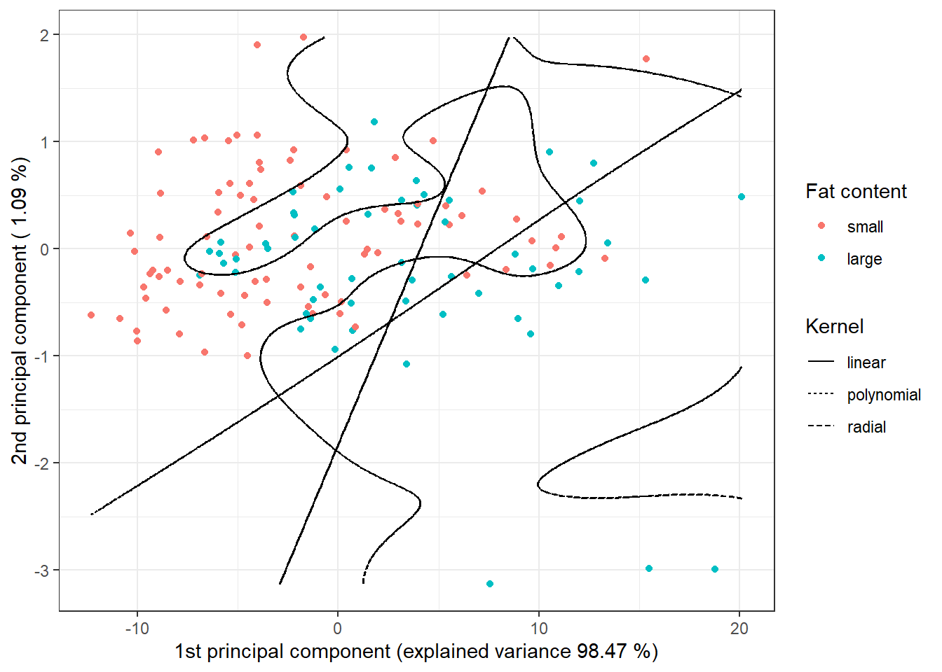 

Figure 3.4: Scores of the first two principal components, color-coded according to class membership. The decision boundary (line or curves in the plane of the first two principal components) between classes is shown in black, constructed using the SVM method.

Code

Res <- data.frame(model = c('SVM linear - PCA', 
                            'SVM poly - PCA', 
                            'SVM rbf - PCA'), 
                  Err.train = 1 - c(presnost.train.l, presnost.train.p, presnost.train.r),
                  Err.test = 1 - c(presnost.test.l, presnost.test.p, presnost.test.r))

RESULTS <- rbind(RESULTS, Res)

6.3.7.4 Basis Coefficients

Finally, we use a B-spline basis to express the functions. For all three kernels, we examine the values of hyperparameter \(C\) in the interval \([10^{-3}, 10^{3}]\). For the polynomial kernel, we fix the hyperparameter \(p\) at 3, as other integer values do not yield nearly as good results. On the other hand, for the radial kernel, we again use 10-fold CV to select the optimal value of hyperparameter \(\gamma\), considering values in the interval \([10^{-4}, 10^{0}]\). We set coef0 \(= 1\).

Code

set.seed(42)

# gamma values to consider
gamma.cv <- 10^seq(-4, 0, length = 5)
C.cv <- 10^seq(-3, 3, length = 7)
p.cv <- 3
coef0 <- 1

# list with three components...array for each kernel -> linear, poly, radial
# empty matrix to store individual results
# columns hold accuracy values for given
# rows represent values for given gamma, and layers correspond to folds
CV.results <- list(
  SVM.l = array(NA, dim = c(length(C.cv), k_cv)),
  SVM.p = array(NA, dim = c(length(C.cv), length(p.cv), k_cv)),
  SVM.r = array(NA, dim = c(length(C.cv), length(gamma.cv), k_cv))
)

# first iterate through values of C
for (C in C.cv) {
  # iterate over individual folds
  for (index_cv in 1:k_cv) {
    # define test and training parts for CV
    fold <- folds[[index_cv]]
    cv_sample <- 1:dim(grid.data)[1] %in% fold
    
    data.Bbasis.train.cv <- as.data.frame(data.Bbasis.train[cv_sample, ])
    data.Bbasis.test.cv <- as.data.frame(data.Bbasis.train[!cv_sample, ])
    
    ## LINEAR KERNEL
    # model creation
    clf.SVM.l <- svm(Y ~ ., data = data.Bbasis.train.cv,
                     type = 'C-classification',
                     scale = TRUE,
                     cost = C,
                     kernel = 'linear')
    
    # accuracy on validation data
    predictions.test.l <- predict(clf.SVM.l, newdata = data.Bbasis.test.cv)
    presnost.test.l <- table(data.Bbasis.test.cv$Y, predictions.test.l) |>
      prop.table() |> diag() |> sum()
    
    # insert accuracies in positions for given C and fold
    CV.results$SVM.l[(1:length(C.cv))[C.cv == C], 
                     index_cv] <- presnost.test.l
    
    ## POLYNOMIAL KERNEL
    for (p in p.cv) {
      # model creation
      clf.SVM.p <- svm(Y ~ ., data = data.Bbasis.train.cv,
                       type = 'C-classification',
                       scale = TRUE,
                       cost = C,
                       coef0 = coef0,
                       degree = p,
                       kernel = 'polynomial')
      
      # accuracy on validation data
      predictions.test.p <- predict(clf.SVM.p, 
                                    newdata = data.Bbasis.test.cv)
      presnost.test.p <- table(data.Bbasis.test.cv$Y, predictions.test.p) |>
        prop.table() |> diag() |> sum()
      
      # insert accuracies in positions for given C, p, and fold
      CV.results$SVM.p[(1:length(C.cv))[C.cv == C], 
                       (1:length(p.cv))[p.cv == p],
                       index_cv] <- presnost.test.p
    }
        
    ## RADIAL KERNEL
    for (gamma in gamma.cv) {
      # model creation
      clf.SVM.r <- svm(Y ~ ., data = data.Bbasis.train.cv,
                       type = 'C-classification',
                       scale = TRUE,
                       cost = C,
                       gamma = gamma,
                       kernel = 'radial')
      
      # accuracy on validation data
      predictions.test.r <- predict(clf.SVM.r, 
                                    newdata = data.Bbasis.test.cv)
      presnost.test.r <- table(data.Bbasis.test.cv$Y, predictions.test.r) |>
        prop.table() |> diag() |> sum()
      
      # insert accuracies in positions for given C, gamma, and fold
      CV.results$SVM.r[(1:length(C.cv))[C.cv == C], 
                       (1:length(gamma.cv))[gamma.cv == gamma],
                       index_cv] <- presnost.test.r
    }
  }
}

Now we will average the results from 10-fold cross-validation so that we have a single estimate of validation error for each hyperparameter value (or combination of values). We will also determine the optimal values for each of the hyperparameters.

Code

# let's calculate the average accuracies for individual C over folds
## Linear kernel
CV.results$SVM.l <- apply(CV.results$SVM.l, 1, mean)
## Polynomial kernel
CV.results$SVM.p <- apply(CV.results$SVM.p, c(1, 2), mean)
## Radial kernel
CV.results$SVM.r <- apply(CV.results$SVM.r, c(1, 2), mean)

C.opt <- c(which.max(CV.results$SVM.l), 
           which.max(CV.results$SVM.p) %% length(C.cv), 
           which.max(CV.results$SVM.r) %% length(C.cv))
C.opt[C.opt == 0] <- length(C.cv)
C.opt <- C.cv[C.opt]

gamma.opt <- which.max(t(CV.results$SVM.r)) %% length(gamma.cv)
gamma.opt[gamma.opt == 0] <- length(gamma.cv)
gamma.opt <- gamma.cv[gamma.opt]

p.opt <- which.max(t(CV.results$SVM.p)) %% length(p.cv)
p.opt[p.opt == 0] <- length(p.cv)
p.opt <- p.cv[p.opt]

presnost.opt.cv <- c(max(CV.results$SVM.l), 
                     max(CV.results$SVM.p),
                     max(CV.results$SVM.r))

Let’s look at how the optimal values turned out. For linear kernel, the optimal value of \(C\) is 10, for polynomial kernel, \(C\) is 100, and for radial kernel, we have two optimal values; for \(C\), the optimal value is 100 and for \(\gamma\), it is 0.01. The validation errors are 0.0195833 for linear, 0.0325 for polynomial, and 0.0392262 for radial kernel.

Finally, we can build the final classifiers on the entire training data with hyperparameter values determined using 10-fold CV. We will also determine the errors on the test and training data.

Code

# building the models
clf.SVM.l.Bbasis <- svm(Y ~ ., data = data.Bbasis.train,
                        type = 'C-classification',
                        scale = TRUE,
                        cost = C.opt[1],
                        kernel = 'linear')

clf.SVM.p.Bbasis <- svm(Y ~ ., data = data.Bbasis.train,
                        type = 'C-classification',
                        scale = TRUE,
                        cost = C.opt[2],
                        degree = p.opt,
                        coef0 = coef0,
                        kernel = 'polynomial')

clf.SVM.r.Bbasis <- svm(Y ~ ., data = data.Bbasis.train,
                        type = 'C-classification',
                        scale = TRUE,
                        cost = C.opt[3],
                        gamma = gamma.opt,
                        kernel = 'radial')

# accuracy on training data
predictions.train.l <- predict(clf.SVM.l.Bbasis, newdata = data.Bbasis.train)
presnost.train.l <- table(Y.train, predictions.train.l) |>
  prop.table() |> diag() |> sum()

predictions.train.p <- predict(clf.SVM.p.Bbasis, newdata = data.Bbasis.train)
presnost.train.p <- table(Y.train, predictions.train.p) |>
  prop.table() |> diag() |> sum()

predictions.train.r <- predict(clf.SVM.r.Bbasis, newdata = data.Bbasis.train)
presnost.train.r <- table(Y.train, predictions.train.r) |>
  prop.table() |> diag() |> sum()
  
# accuracy on test data
predictions.test.l <- predict(clf.SVM.l.Bbasis, newdata = data.Bbasis.test)
presnost.test.l <- table(Y.test, predictions.test.l) |>
  prop.table() |> diag() |> sum()

predictions.test.p <- predict(clf.SVM.p.Bbasis, newdata = data.Bbasis.test)
presnost.test.p <- table(Y.test, predictions.test.p) |>
  prop.table() |> diag() |> sum()

predictions.test.r <- predict(clf.SVM.r.Bbasis, newdata = data.Bbasis.test)
presnost.test.r <- table(Y.test, predictions.test.r) |>
  prop.table() |> diag() |> sum()

The error rate of the SVM method applied to the base coefficients on the training data is 0.67 % for the linear kernel, 0.67 % for the polynomial kernel, and 1.33 % for the Gaussian kernel. On the test data, the error rate is 6.1538 % for the linear kernel, 9.2308 % for the polynomial kernel, and 6.1538 % for the radial kernel.

Code

Res <- data.frame(model = c('SVM linear - Bbasis', 
                            'SVM poly - Bbasis', 
                            'SVM rbf - Bbasis'), 
                  Err.train = 1 - c(presnost.train.l, presnost.train.p, presnost.train.r),
                  Err.test = 1 - c(presnost.test.l, presnost.test.p, presnost.test.r))

RESULTS <- rbind(RESULTS, Res)

6.3.7.5 Projection onto B-spline Basis

Another way to apply the classic SVM method to functional data is to project the original data onto some \(d\)-dimensional subspace of our Hilbert space \(\mathcal H\), denoted as \(V_d\). Let’s assume that this subspace \(V_d\) has an orthonormal basis \(\{\Psi_j\}_{j = 1, \dots, d}\). We define the transformation \(P_{V_d}\) as the orthogonal projection onto the subspace \(V_d\), which we can express as

\[ P_{V_d} (x) = \sum_{j = 1}^d \langle x, \Psi_j \rangle \Psi_j. \]

Now we can use the coefficients from the orthogonal projection for classification, applying standard SVM to the vectors \(\left( \langle x, \Psi_1 \rangle, \dots, \langle x, \Psi_d \rangle\right)^\top\). By using this transformation, we have defined a new, so-called adapted kernel, which consists of the orthogonal projection \(P_{V_d}\) and the kernel function of the standard support vector machine. Thus, we have the (adapted) kernel \(Q(x_i, x_j) = K(P_{V_d}(x_i), P_{V_d}(x_j))\). This is a dimensionality reduction method that we can call filtering.

For the actual projection, we will use the project.basis() function from the fda library in R. Its input will be a matrix of the original discrete (unsmoothed) data, the values in which we measure values in the original data matrix, and the basis object onto which we want to project the data. We choose to project onto a B-spline basis because the use of a Fourier basis is not suitable for our non-periodic data.

The dimension \(d\) is chosen either based on some prior expert knowledge or through cross-validation. In our case, we will determine the optimal dimension of the subspace \(V_d\) using \(k\)-fold cross-validation (with \(k \ll n\) due to the computational intensity of the method; commonly \(k = 5\) or \(k = 10\) is chosen). We require B-splines of order 4, and the relationship for the number of basis functions is given by

\[ n_{basis} = n_{breaks} + n_{order} - 2, \]

where \(n_{breaks}\) is the number of knots and \(n_{order} = 4\). However, in R, the value of \(n_{basis}\) must be at least \(n_{order} = 4\), and for large values of \(n_{basis}\), we risk overfitting the model. Thus, we choose a maximum of \(n_{basis}\) to be a smaller number, say 20.

Code

k_cv <- 10 # k-fold CV

# Values for B-spline basis
rangeval <- range(t)
norder <- 4
n_basis_min <- norder
n_basis_max <- 20

dimensions <- n_basis_min:n_basis_max # All dimensions we want to try

# Split the training data into k parts
folds <- createMultiFolds(1:sum(split), k = k_cv, time = 1)

# List with three components ... matrices for each kernel -> linear, poly, radial
# Empty matrix to store results
# Columns will be accuracy values for a given part of the training set
# Rows will correspond to values for a given dimension
CV.results <- list(SVM.l = matrix(NA, nrow = length(dimensions), ncol = k_cv),
                   SVM.p = matrix(NA, nrow = length(dimensions), ncol = k_cv),
                   SVM.r = matrix(NA, nrow = length(dimensions), ncol = k_cv))

for (d in dimensions) {
  # Basis object
  bbasis <- create.bspline.basis(rangeval = rangeval, 
                                 nbasis = d)
  
  # Projecting discrete data onto B-spline basis of dimension d
  Projection <- project.basis(y = XX, # Matrix of discrete data
                              argvals = t, # Vector of arguments
                              basisobj = bbasis) # Basis object
  
  # Splitting into training and testing data for CV
  XX.train <- subset(t(Projection), split == TRUE)
  
  for (index_cv in 1:k_cv) {
    # Define test and training parts for CV
    fold <- folds[[index_cv]]
    cv_sample <- 1:dim(XX.train)[1] %in% fold
    
    data.projection.train.cv <- as.data.frame(XX.train[cv_sample, ])
    data.projection.train.cv$Y <- factor(Y.train[cv_sample])
    
    data.projection.test.cv <- as.data.frame(XX.train[!cv_sample, ])
    Y.test.cv <- Y.train[!cv_sample]
    data.projection.test.cv$Y <- factor(Y.test.cv)
  
    # Model construction
    clf.SVM.l.projection <- svm(Y ~ ., data = data.projection.train.cv,
                            type = 'C-classification',
                            scale = TRUE,
                            kernel = 'linear')
    
    clf.SVM.p.projection <- svm(Y ~ ., data = data.projection.train.cv,
                            type = 'C-classification',
                            scale = TRUE,
                            coef0 = coef0,
                            kernel = 'polynomial')
    
    clf.SVM.r.projection <- svm(Y ~ ., data = data.projection.train.cv,
                            type = 'C-classification',
                            scale = TRUE,
                            kernel = 'radial')
      
    # Accuracy on validation data
    ## Linear kernel
    predictions.test.l <- predict(clf.SVM.l.projection,
                                  newdata = data.projection.test.cv)
    presnost.test.l <- table(Y.test.cv, predictions.test.l) |>
      prop.table() |> diag() |> sum()
    ## Polynomial kernel
    predictions.test.p <- predict(clf.SVM.p.projection, 
                                  newdata = data.projection.test.cv)
    presnost.test.p <- table(Y.test.cv, predictions.test.p) |>
      prop.table() |> diag() |> sum()
    ## Radial kernel
    predictions.test.r <- predict(clf.SVM.r.projection,
                                  newdata = data.projection.test.cv)
    presnost.test.r <- table(Y.test.cv, predictions.test.r) |>
      prop.table() |> diag() |> sum()
    
    # Store accuracies in positions for given d and fold
    CV.results$SVM.l[d - min(dimensions) + 1, index_cv] <- presnost.test.l
    CV.results$SVM.p[d - min(dimensions) + 1, index_cv] <- presnost.test.p
    CV.results$SVM.r[d - min(dimensions) + 1, index_cv] <- presnost.test.r
  }
}
  
# Compute average accuracies for each d across folds
for (n_method in 1:length(CV.results)) {
  CV.results[[n_method]] <- apply(CV.results[[n_method]], 1, mean)
}

d.opt <- c(which.max(CV.results$SVM.l) + n_basis_min - 1, 
           which.max(CV.results$SVM.p) + n_basis_min - 1, 
           which.max(CV.results$SVM.r) + n_basis_min - 1)
presnost.opt.cv <- c(max(CV.results$SVM.l), 
                     max(CV.results$SVM.p),
                     max(CV.results$SVM.r))
data.frame(d_opt = d.opt, ERR = 1 - presnost.opt.cv,
           row.names = c('linear', 'poly', 'radial'))

##        d_opt        ERR
## linear     9 0.01958333
## poly       7 0.03297619
## radial     6 0.14125000

We see that the optimal value of the parameter \(d\) is 9 for the linear kernel with an error rate calculated using 10-fold CV of 0.0196, 7 for the polynomial kernel with an error rate calculated using 10-fold CV of 0.033, and 6 for the radial kernel with an error rate of 0.1412.

For clarity, let’s plot the validation error rates as a function of the dimension \(d\).

Code

CV.results <- data.frame(d = dimensions |> rep(3), 
                         CV = c(CV.results$SVM.l, 
                                CV.results$SVM.p, 
                                CV.results$SVM.r),
                         Kernel = rep(c('linear', 'polynomial', 'radial'), 
                                      each = length(dimensions)) |> factor())
CV.results |> ggplot(aes(x = d, y = 1 - CV, colour = Kernel)) + 
  geom_line(linetype = 'dashed') + 
  geom_point(size = 1.5) + 
  geom_point(data = data.frame(d.opt,
                               presnost.opt.cv),
             aes(x = d.opt, y = 1 - presnost.opt.cv), colour = 'black', size = 2) +
  theme_bw() + 
  labs(x = bquote(paste(d)),
       y = 'Validation Error',
       colour = 'Kernel') + 
  theme(legend.position = "bottom") + 
  scale_x_continuous(breaks = dimensions)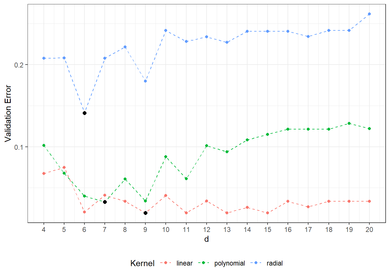

Figure 1.23: Dependence of validation error on the dimension of the subspace \(V_d\), separately for all three considered kernels in the SVM method. The optimal values of the dimension \(V_d\) for each kernel function are marked with black dots.

Now we can train individual classifiers on all training data and examine their performance on the test data. For each kernel function, we choose the dimension of the subspace onto which we project based on the results of cross-validation.

In the variable Projection, we have stored the matrix of coefficients for the orthogonal projection, which is given by

\[ \texttt{Projection} = \begin{pmatrix} \langle x_1, \Psi_1 \rangle & \langle x_2, \Psi_1 \rangle & \cdots & \langle x_n, \Psi_1 \rangle\\ \langle x_1, \Psi_2 \rangle & \langle x_2, \Psi_2 \rangle & \cdots & \langle x_n, \Psi_2 \rangle\\ \vdots & \vdots & \ddots & \vdots \\ \langle x_1, \Psi_d \rangle & \langle x_2, \Psi_d \rangle & \dots & \langle x_n, \Psi_d \rangle \end{pmatrix}_{d \times n}. \]

Code

# Prepare a data table to store results
Res <- data.frame(model = c('SVM linear - projection', 
                            'SVM poly - projection', 
                            'SVM rbf - projection'), 
                  Err.train = NA,
                  Err.test = NA)

# Loop through the individual kernels
for (kernel_number in 1:3) {
  kernel_type <- c('linear', 'polynomial', 'radial')[kernel_number]
  # Create the base object
  bbasis <- create.bspline.basis(rangeval = rangeval, 
                                 nbasis = d.opt[kernel_number])
  
  # Project discrete data onto the B-spline basis
  Projection <- project.basis(y = XX, # matrix of discrete data
                              argvals = t, # vector of arguments
                              basisobj = bbasis) # basis object
  
  # Split into training and testing data
  XX.train <- subset(t(Projection), split == TRUE)
  XX.test <- subset(t(Projection), split == FALSE)
  
  data.projection.train <- as.data.frame(XX.train)
  data.projection.train$Y <- factor(Y.train)
  
  data.projection.test <- as.data.frame(XX.test)
  data.projection.test$Y <- factor(Y.test)
  
  # Build the model
  clf.SVM.projection <- svm(Y ~ ., data = data.projection.train,
                            type = 'C-classification',
                            scale = TRUE,
                            coef0 = coef0,
                            kernel = kernel_type)
  
  # Accuracy on training data
  predictions.train <- predict(clf.SVM.projection, newdata = data.projection.train)
  presnost.train <- table(Y.train, predictions.train) |>
    prop.table() |> diag() |> sum()
    
  # Accuracy on testing data
  predictions.test <- predict(clf.SVM.projection, newdata = data.projection.test)
  presnost.test <- table(Y.test, predictions.test) |>
    prop.table() |> diag() |> sum()
  
  # Store results
  Res[kernel_number, c(2, 3)] <- 1 - c(presnost.train, presnost.test)
}

The error rate of the SVM method applied to the basis coefficients on the training data is therefore 2 % for the linear kernel, 2.67 % for the polynomial kernel, and 9.33 % for the Gaussian kernel. The error rate of the method on the test data is then 6.15 % for the linear kernel, 6.15 % for the polynomial kernel, and 10.77 % for the radial kernel.

Code

RESULTS <- rbind(RESULTS, Res)

6.3.7.6 RKHS + SVM

In this section, we will explore another way to utilize the support vector machine (SVM) method for the classification of functional data. Again, we will follow the familiar principle of expressing functional data as finite-dimensional objects, to which we then apply the traditional SVM method.

However, this time we will use SVM for the representation of functional data itself through a certain finite-dimensional object. As the name suggests, it combines two concepts: the support vector machine and a space known in English literature as the Reproducing Kernel Hilbert Space (RKHS). The key concept for this space is the kernel.

6.3.7.6.1 Implementation of the method in R

From the last part of Theorem 1.3, we derive how to compute the representations of curves in practice. We will work with discretized data after smoothing the curves. First, let’s define the kernel for the RKHS space. We will use the Gaussian kernel with the parameter \(\gamma\). The value of this hyperparameter significantly affects the behavior and success of the method, so we must pay special attention to its choice (we will select it using cross-validation).

After trying several options, good hyperparameter choices appear to be \(\varepsilon = 0.01\) and \(C = 1\). Due to computational demands, we will not estimate these hyperparameters using CV.

Code

eps <- 0.01
C <- 1 

6.3.7.6.1.1 Gaussian Kernel

Code

# Remove the last column, which contains the values of Y
data.RKHS <- grid.data[, -dim(grid.data)[2]] |> t()
# Add the test data
data.RKHS <- cbind(data.RKHS, grid.data.test[, -dim(grid.data.test)[2]] |> t())

# Kernel and kernel matrix ... Gaussian with parameter gamma
Gauss.kernel <- function(x, y, gamma) {
  return(exp(-gamma * norm(c(x - y) |> t(), type = 'F')))
}

Kernel.RKHS <- function(x, gamma) {
  K <- matrix(NA, ncol = length(x), nrow = length(x))
  for(i in 1:nrow(K)) {
    for(j in 1:ncol(K)) {
      K[i, j] <- Gauss.kernel(x = x[i], y = x[j], gamma = gamma)
    }
  }
  return(K)
}

Now let’s compute the matrix \(K_S\) and its eigenvalues and corresponding eigenvectors.

Code

# Compute the matrix K
gamma <- 0.1 # fixed value for gamma; we will determine the optimal value using CV
K <- Kernel.RKHS(t.seq, gamma = gamma)

# Determine eigenvalues and eigenvectors
Eig <- eigen(K)
eig.vals <- Eig$values
eig.vectors <- Eig$vectors

To compute the coefficients in the representation of curves, that is, the calculation of vectors \(\hat{\boldsymbol \lambda}_l^* = \left( \hat\lambda_{1l}^*, \dots, \hat\lambda_{\hat d l}^*\right)^\top, l = 1, 2, \dots, n\), we also need the coefficients from SVM. Unlike the classification problem, we are now dealing with a regression problem since we are trying to express our observed curves in some (chosen by us via the kernel \(K\)) basis. Thus, we will use the Support Vector Regression method, from which we will subsequently obtain the coefficients \(\alpha_{il}\).

Code

# Determine coefficients alpha from SVM
alpha.RKHS <- matrix(0, nrow = dim(data.RKHS)[1],
                     ncol = dim(data.RKHS)[2]) # empty object

# Model
for(i in 1:dim(data.RKHS)[2]) {
  df.svm <- data.frame(x = t.seq,
                       y = data.RKHS[, i])
  svm.RKHS <- svm(y ~ x, data = df.svm, 
                  kernel = 'radial',
                  type = 'eps-regression',
                  epsilon = eps,
                  cost = C,
                  gamma = gamma)
  # Determine alpha
  alpha.RKHS[svm.RKHS$index, i] <- svm.RKHS$coefs # replace zeros with coefficients
}

We can now compute the representations of the individual curves. First, let’s set \(\hat d\) to the full dimension, that is, \(\hat d = m ={}\) 101, and then we will determine the optimal \(\hat d\) using cross-validation.

Code

# d
d.RKHS <- dim(alpha.RKHS)[1]

# Determine the vector lambda
Lambda.RKHS <- matrix(NA, 
                      ncol = dim(data.RKHS)[2], 
                      nrow = d.RKHS) # create an empty object

# Compute the representation
for(l in 1:dim(data.RKHS)[2]) {
  Lambda.RKHS[, l] <- (t(eig.vectors[, 1:d.RKHS]) %*% alpha.RKHS[, l]) * eig.vals[1:d.RKHS]
}

Now we have stored in the matrix Lambda.RKHS the vectors \(\hat{\boldsymbol \lambda}_l^*, l = 1, 2, \dots, n\) for each curve in the columns. We will use these vectors as a representation of the given curves and classify the data according to this discretization.

Code

# Split into training and testing data
XX.train <- Lambda.RKHS[, 1:dim(grid.data)[1]]
XX.test <- Lambda.RKHS[, (dim(grid.data)[1] + 1):dim(Lambda.RKHS)[2]]

# Prepare a data table to store results
Res <- data.frame(model = c('SVM linear - RKHS', 
                             'SVM poly - RKHS', 
                             'SVM rbf - RKHS'), 
                  Err.train = NA,
                  Err.test = NA)

# Iterate over individual kernels
for (kernel_number in 1:3) {
  kernel_type <- c('linear', 'polynomial', 'radial')[kernel_number]

  data.RKHS.train <- as.data.frame(t(XX.train))
  data.RKHS.train$Y <- factor(Y.train)
  
  data.RKHS.test <- as.data.frame(t(XX.test))
  data.RKHS.test$Y <- factor(Y.test)
  
  # Build the model
  clf.SVM.RKHS <- svm(Y ~ ., data = data.RKHS.train,
                      type = 'C-classification',
                      cost = C,
                      coef0 = coef0,
                      scale = TRUE,
                      kernel = kernel_type)
  
  # Accuracy on training data
  predictions.train <- predict(clf.SVM.RKHS, newdata = data.RKHS.train)
  accuracy.train <- table(Y.train, predictions.train) |>
    prop.table() |> diag() |> sum()
    
  # Accuracy on testing data
  predictions.test <- predict(clf.SVM.RKHS, newdata = data.RKHS.test)
  accuracy.test <- table(Y.test, predictions.test) |>
    prop.table() |> diag() |> sum()
  
  # Store results
  Res[kernel_number, c(2, 3)] <- 1 - c(accuracy.train, accuracy.test)
}

Table 6.1: Summary of SVM method results combined with RKHS on simulated data. \(\widehat{Err}_{train}\) denotes the estimate of training error, and \(\widehat{Err}_{test}\) denotes the testing error estimate.

Model	\(\widehat{Err}_{train}\quad\quad\quad\quad\quad\)	\(\widehat{Err}_{test}\quad\quad\quad\quad\quad\)
SVM linear - RKHS	0.0133	0.1231
SVM poly - RKHS	0.0267	0.0308
SVM rbf - RKHS	0.0400	0.0308

We see that the model classifies the training data very well for all three kernels, while its success on the testing data is not good for the linear kernel. Therefore, we will use cross-validation to determine the optimal values for \(\gamma\) and \(d\).

Code

# Split training data into k parts
folds <- createMultiFolds(1:sum(split), k = k_cv, time = 1)
# Remove the last column which contains the values of Y
data.RKHS <- grid.data[, -dim(grid.data)[2]] |> t()

# Hyperparameter values to iterate over
dimensions <- 3:30 # reasonable range of values for d
gamma.cv <- 10^seq(-2, 2, length = 15)

# List with three components... array for individual kernels -> linear, poly, radial
# Empty matrix to store individual results
# Columns will contain accuracy values for given
# Rows will contain values for given gamma, and layers correspond to folds
dim.names <- list(gamma = paste0('gamma:', round(gamma.cv, 3)),
                  d = paste0('d:', dimensions),
                  CV = paste0('cv:', 1:k_cv))

CV.results <- list(
  SVM.l = array(NA, dim = c(length(gamma.cv), length(dimensions), k_cv),
                dimnames = dim.names),
  SVM.p = array(NA, dim = c(length(gamma.cv), length(dimensions), k_cv),
                dimnames = dim.names),
  SVM.r = array(NA, dim = c(length(gamma.cv), length(dimensions), k_cv),
                dimnames = dim.names))

Code

# Cross-validation itself
for (gamma in gamma.cv) {
  K <- Kernel.RKHS(t.seq, gamma = gamma)
  Eig <- eigen(K)
  eig.vals <- Eig$values
  eig.vectors <- Eig$vectors
  alpha.RKHS <- matrix(0, nrow = dim(data.RKHS)[1], ncol = dim(data.RKHS)[2]) 
  
  # Model
  for(i in 1:dim(data.RKHS)[2]) {
    df.svm <- data.frame(x = t.seq,
                         y = data.RKHS[, i])
    svm.RKHS <- svm(y ~ x, data = df.svm, 
                    kernel = 'radial',
                    type = 'eps-regression',
                    epsilon = eps,
                    cost = C,
                    gamma = gamma)
    alpha.RKHS[svm.RKHS$index, i] <- svm.RKHS$coefs 
  }
  
  # Iterate over dimensions
  for(d.RKHS in dimensions) {
    Lambda.RKHS <- matrix(NA, 
                          ncol = dim(data.RKHS)[2], 
                          nrow = d.RKHS) 
    # Compute representation
    for(l in 1:dim(data.RKHS)[2]) {
      Lambda.RKHS[, l] <- (t(eig.vectors[, 1:d.RKHS]) %*% 
                             alpha.RKHS[, l]) * eig.vals[1:d.RKHS]
    }
    # Iterate over folds
    for (index_cv in 1:k_cv) {
      # Define testing and training parts for CV
      fold <- folds[[index_cv]]
      # Split into training and validation data
      XX.train <- Lambda.RKHS[, fold]
      XX.test <- Lambda.RKHS[, !(1:dim(Lambda.RKHS)[2] %in% fold)]
      # Prepare a data table to store results
      Res <- data.frame(model = c('SVM linear - RKHS', 
                                   'SVM poly - RKHS', 
                                   'SVM rbf - RKHS'), 
                        Err.test = NA)
      # Iterate over individual kernels
      for (kernel_number in 1:3) {
        kernel_type <- c('linear', 'polynomial', 'radial')[kernel_number]
      
        data.RKHS.train <- as.data.frame(t(XX.train))
        data.RKHS.train$Y <- factor(Y.train[fold])
        
        data.RKHS.test <- as.data.frame(t(XX.test))
        data.RKHS.test$Y <- factor(Y.train[!(1:dim(Lambda.RKHS)[2] %in% fold)])
        
        # Build the model
        clf.SVM.RKHS <- svm(Y ~ ., data = data.RKHS.train,
                            type = 'C-classification',
                            scale = TRUE,
                            cost = C,
                            coef0 = coef0,
                            kernel = kernel_type)
        
        # Accuracy on validation data
        predictions.test <- predict(clf.SVM.RKHS, newdata = data.RKHS.test)
        accuracy.test <- table(data.RKHS.test$Y, predictions.test) |>
          prop.table() |> diag() |> sum()
        
        # Store results
        Res[kernel_number, 2] <- 1 - accuracy.test
      }
      # Insert accuracies into positions for given d, gamma, and fold
      CV.results$SVM.l[paste0('gamma:', round(gamma, 3)), 
                       d.RKHS - min(dimensions) + 1, 
                       index_cv] <- Res[1, 2]
      CV.results$SVM.p[paste0('gamma:', round(gamma, 3)), 
                       d.RKHS - min(dimensions) + 1, 
                       index_cv] <- Res[2, 2]
      CV.results$SVM.r[paste0('gamma:', round(gamma, 3)), 
                       d.RKHS - min(dimensions) + 1, 
                       index_cv] <- Res[3, 2]
    }
  }
}

Code

# We calculate the average accuracies for each method across folds
for (n_method in 1:length(CV.results)) {
  CV.results[[n_method]] <- apply(CV.results[[n_method]], c(1, 2), mean)
}

gamma.opt <- c(which.min(CV.results$SVM.l) %% length(gamma.cv), 
               which.min(CV.results$SVM.p) %% length(gamma.cv), 
               which.min(CV.results$SVM.r) %% length(gamma.cv))
gamma.opt[gamma.opt == 0] <- length(gamma.cv)
gamma.opt <- gamma.cv[gamma.opt]

d.opt <- c(which.min(t(CV.results$SVM.l)) %% length(dimensions), 
           which.min(t(CV.results$SVM.p)) %% length(dimensions), 
           which.min(t(CV.results$SVM.r)) %% length(dimensions))
d.opt[d.opt == 0] <- length(dimensions)
d.opt <- dimensions[d.opt]

err.opt.cv <- c(min(CV.results$SVM.l), 
                 min(CV.results$SVM.p),
                 min(CV.results$SVM.r))
df.RKHS.res <- data.frame(d = d.opt, gamma = gamma.opt, CV = err.opt.cv,
           Kernel = c('linear', 'polynomial', 'radial') |> factor(),
           row.names = c('linear', 'poly', 'radial'))

Table 6.2: Summary of cross-validation results for the SVM method combined with RKHS on simulated data. \(\widehat{Err}_{train}\) denotes the estimate of training error and \(\widehat{Err}_{test}\) the test error.

	\(\quad\quad\quad\quad\quad d\)	\(\quad\quad\quad\quad\quad\gamma\)	\(\widehat{Err}_{cross\_validation}\)	Model
linear	11	1.0000	0	linear
poly	27	1.0000	0	polynomial
radial	30	3.7276	0	radial

We see that the optimal parameter values are \(d={}\) 11 and \(\gamma={}\) 1 for the linear kernel with an error value calculated using 10-fold CV 0, \(d={}\) 27 and \(\gamma={}\) 1 for the polynomial kernel with an error value calculated using 10-fold CV 0, and \(d={}\) 30 and \(\gamma={}\) 3.7276 for the radial kernel with an error value of 0. For interest, let’s plot the validation error function in relation to the dimension \(d\) and the hyperparameter \(\gamma\) values.

Code

CV.results.plot <- data.frame(d = rep(dimensions |> rep(3), each = length(gamma.cv)), 
                              gamma = rep(gamma.cv, length(dimensions)) |> rep(3),
                               CV = c(c(CV.results$SVM.l), 
                                      c(CV.results$SVM.p), 
                                      c(CV.results$SVM.r)),
                               Kernel = rep(c('linear', 'polynomial', 'radial'), 
                                            each = length(dimensions) * 
                                              length(gamma.cv)) |> factor())
CV.results.plot |> 
  ggplot(aes(x = d, y = gamma, z = CV)) + 
  geom_contour_filled() +
  scale_y_continuous(trans='log10') +
  facet_wrap(~Kernel) +
  theme_bw() + 
  labs(x = expression(d),
       y = expression(gamma)) + 
  scale_fill_brewer(palette = "Spectral") + 
  geom_point(data = df.RKHS.res, aes(x = d, y = gamma),
             size = 5, pch = '+')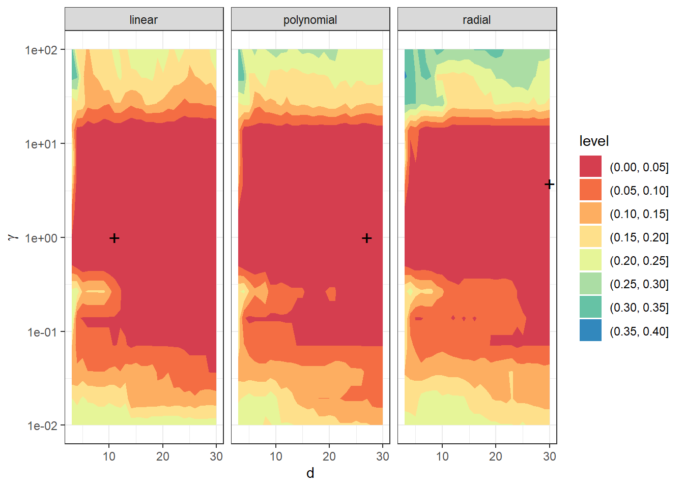

Figure 6.10: Dependence of validation error on the choice of hyperparameters \(d\) and \(\gamma\), separately for all three considered kernels in the SVM method.

In the above graphs, we observe how the validation error varied depending on the hyperparameter values \(d\) and \(\gamma\). Notably, in all three graphs for the individual kernels, significant horizontal structures are apparent. From this, we can draw significant theoretical and practical insights— the considered classification method (projection onto RKHS using SVM + SVM classification) is robust to the choice of hyperparameter \(d\) (i.e., a small change in this parameter value does not lead to a significant deterioration in validation error), while we must be very cautious with the choice of hyperparameter \(\gamma\) (even a small change in its value can lead to a large change in validation error). This behavior is most evident with the Gaussian kernel.

Since we have already found the optimal values for the hyperparameters, we can construct the final models and assess their classification success on the test data.

Code

# We remove the last column containing the Y values
data.RKHS <- grid.data[, -dim(grid.data)[2]] |> t()
# We also add the test data
data.RKHS <- cbind(data.RKHS, grid.data.test[, -dim(grid.data.test)[2]] |> t())

Code

# Prepare a data table for storing results
Res <- data.frame(model = c('SVM linear - RKHS - radial', 
                            'SVM poly - RKHS - radial', 
                            'SVM rbf - RKHS - radial'), 
                  Err.train = NA,
                  Err.test = NA)

# Iterate through the individual kernels
for (kernel_number in 1:3) {
  # Calculate the K matrix
  gamma <- gamma.opt[kernel_number] # gamma value from CV
  K <- Kernel.RKHS(t.seq, gamma = gamma)
  
  # Determine eigenvalues and eigenvectors
  Eig <- eigen(K)
  eig.vals <- Eig$values
  eig.vectors <- Eig$vectors
  # Determine coefficients alpha from SVM
  alpha.RKHS <- matrix(0, nrow = dim(data.RKHS)[1],
                       ncol = dim(data.RKHS)[2]) # empty object
  
  # Model
  for(i in 1:dim(data.RKHS)[2]) {
    df.svm <- data.frame(x = t.seq,
                         y = data.RKHS[, i])
    svm.RKHS <- svm(y ~ x, data = df.svm, 
                    kernel = 'radial',
                    type = 'eps-regression',
                    epsilon = eps,
                    cost = C,
                    gamma = gamma)
    # Determine alpha
    alpha.RKHS[svm.RKHS$index, i] <- svm.RKHS$coefs # replace zeros with coefficients
  }
  # d
  d.RKHS <- d.opt[kernel_number]
  
  # Determine the lambda vector
  Lambda.RKHS <- matrix(NA, 
                        ncol = dim(data.RKHS)[2], 
                        nrow = d.RKHS) # create empty object
  
  # Calculate representation
  for(l in 1:dim(data.RKHS)[2]) {
    Lambda.RKHS[, l] <- (t(eig.vectors[, 1:d.RKHS]) %*% alpha.RKHS[, l]) * eig.vals[1:d.RKHS]
  }
  
  # Split into training and test data
  XX.train <- Lambda.RKHS[, 1:dim(grid.data)[1]]
  XX.test <- Lambda.RKHS[, (dim(grid.data)[1] + 1):dim(Lambda.RKHS)[2]]

  kernel_type <- c('linear', 'polynomial', 'radial')[kernel_number]

  data.RKHS.train <- as.data.frame(t(XX.train))
  data.RKHS.train$Y <- factor(Y.train)
  
  data.RKHS.test <- as.data.frame(t(XX.test))
  data.RKHS.test$Y <- factor(Y.test)
  
  # Model building
  clf.SVM.RKHS <- svm(Y ~ ., data = data.RKHS.train,
                      type = 'C-classification',
                      scale = TRUE,
                      cost = C,
                      coef0 = coef0,
                      kernel = kernel_type)
  
  # Accuracy on training data
  predictions.train <- predict(clf.SVM.RKHS, newdata = data.RKHS.train)
  presnost.train <- table(Y.train, predictions.train) |>
    prop.table() |> diag() |> sum()
    
  # Accuracy on test data
  predictions.test <- predict(clf.SVM.RKHS, newdata = data.RKHS.test)
  presnost.test <- table(Y.test, predictions.test) |>
    prop.table() |> diag() |> sum()
  
  # Store results
  Res[kernel_number, c(2, 3)] <- 1 - c(presnost.train, presnost.test)
}

Table 6.3: Summary of SVM method results combined with RKHS on simulated data. \(\widehat{Err}_{train}\) denotes the estimate of training error and \(\widehat{Err}_{test}\) the test error.

Model	\(\widehat{Err}_{train}\quad\quad\quad\quad\quad\)	\(\widehat{Err}_{test}\quad\quad\quad\quad\quad\)
SVM linear - RKHS - radial	0	0.0308
SVM poly - RKHS - radial	0	0.0308
SVM rbf - RKHS - radial	0	0.0154

The error rate of the SVM method combined with the projection onto the Reproducing Kernel Hilbert Space is therefore 0 % on the training data for the linear kernel, 0 % for the polynomial kernel, and 0 % for the Gaussian kernel. On the test data, the error rate of the method is 3.08 % for the linear kernel, 3.08 % for the polynomial kernel, and 1.54 % for the radial kernel.

Code

RESULTS <- rbind(RESULTS, Res)

6.3.7.6.1.2 Polynomial Kernel

Code

# Remove the last column, which contains the Y values
data.RKHS <- grid.data[, -dim(grid.data)[2]] |> t()
# Add test data as well
data.RKHS <- cbind(data.RKHS, grid.data.test[, -dim(grid.data.test)[2]] |> t())

# Kernel and kernel matrix ... polynomial with parameter p
Poly.kernel <- function(x, y, p) {
  return((1 + x * y)^p)
}

Kernel.RKHS <- function(x, p) {
  K <- matrix(NA, ncol = length(x), nrow = length(x))
  for(i in 1:nrow(K)) {
    for(j in 1:ncol(K)) {
      K[i, j] <- Poly.kernel(x = x[i], y = x[j], p)
    }
  }
  return(K)
}

Code

# Split training data into k parts
folds <- createMultiFolds(1:sum(split), k = k_cv, time = 1)
# Remove the last column, which contains the Y values
data.RKHS <- grid.data[, -dim(grid.data)[2]] |> t()

# Hyperparameter values to iterate through
dimensions <- 2:30 # reasonable range for d
poly.cv <- 2:5

# List with three components ... array for individual kernels -> linear, poly, radial
# Empty matrix to store the results
# Columns will be accuracy values for the given parameters
# Rows will correspond to values for p and layers will correspond to folds
dim.names <- list(p = paste0('p:', poly.cv),
                  d = paste0('d:', dimensions),
                  CV = paste0('cv:', 1:k_cv))

CV.results <- list(
  SVM.l = array(NA, dim = c(length(poly.cv), length(dimensions), k_cv),
                dimnames = dim.names),
  SVM.p = array(NA, dim = c(length(poly.cv), length(dimensions), k_cv),
                dimnames = dim.names),
  SVM.r = array(NA, dim = c(length(poly.cv), length(dimensions), k_cv),
                dimnames = dim.names))

Code

# Cross-validation itself
for (p in poly.cv) {
  K <- Kernel.RKHS(t.seq, p = p)
  Eig <- eigen(K)
  eig.vals <- Eig$values
  eig.vectors <- Eig$vectors
  alpha.RKHS <- matrix(0, nrow = dim(data.RKHS)[1], ncol = dim(data.RKHS)[2]) 
  
  # Model
  for(i in 1:dim(data.RKHS)[2]) {
    df.svm <- data.frame(x = t.seq,
                         y = data.RKHS[, i])
    svm.RKHS <- svm(y ~ x, data = df.svm, 
                    kernel = 'polynomial',
                    type = 'eps-regression',
                    coef0 = 1,
                    cost = C,
                    epsilon = eps,
                    degree = p)
    alpha.RKHS[svm.RKHS$index, i] <- svm.RKHS$coefs 
  }
  
  # Iterate through dimensions
  for(d.RKHS in dimensions) {
    Lambda.RKHS <- matrix(NA, 
                          ncol = dim(data.RKHS)[2], 
                          nrow = d.RKHS) 
    # Calculate representation
    for(l in 1:dim(data.RKHS)[2]) {
      Lambda.RKHS[, l] <- (t(eig.vectors[, 1:d.RKHS]) %*% 
                             alpha.RKHS[, l]) * eig.vals[1:d.RKHS]
    }
    # Iterate through folds
    for (index_cv in 1:k_cv) {
      # Define test and training parts for CV
      fold <- folds[[index_cv]]
      # Split into training and validation data
      XX.train <- Lambda.RKHS[, fold]
      XX.test <- Lambda.RKHS[, !(1:dim(Lambda.RKHS)[2] %in% fold)]
      # Prepare a data table to store results
      Res <- data.frame(model = c('SVM linear - RKHS', 
                                  'SVM poly - RKHS', 
                                  'SVM rbf - RKHS'), 
                        Err.test = NA)
      # Iterate through individual kernels
      for (kernel_number in 1:3) {
        kernel_type <- c('linear', 'polynomial', 'radial')[kernel_number]
      
        data.RKHS.train <- as.data.frame(t(XX.train))
        data.RKHS.train$Y <- factor(Y.train[fold])
        
        data.RKHS.test <- as.data.frame(t(XX.test))
        data.RKHS.test$Y <- factor(Y.train[!(1:dim(Lambda.RKHS)[2] %in% fold)])
        
        # Model construction
        clf.SVM.RKHS <- svm(Y ~ ., data = data.RKHS.train,
                            type = 'C-classification',
                            scale = TRUE,
                            cost = C,                    
                            coef0 = 1,
                            gamma = 1,
                            kernel = kernel_type)
        
        # Accuracy on validation data
        predictions.test <- predict(clf.SVM.RKHS, newdata = data.RKHS.test)
        presnost.test <- table(data.RKHS.test$Y, predictions.test) |>
          prop.table() |> diag() |> sum()
        
        # Store results
        Res[kernel_number, 2] <- 1 - presnost.test
      }
      # Store accuracies for the given d, gamma, and fold
      CV.results$SVM.l[paste0('p:', p), 
                       d.RKHS - min(dimensions) + 1, 
                       index_cv] <- Res[1, 2]
      CV.results$SVM.p[paste0('p:', p), 
                       d.RKHS - min(dimensions) + 1, 
                       index_cv] <- Res[2, 2]
      CV.results$SVM.r[paste0('p:', p), 
                       d.RKHS - min(dimensions) + 1, 
                       index_cv] <- Res[3, 2]
    }
  }
}

Code

# Calculate average accuracies for each d across folds
for (n_method in 1:length(CV.results)) {
  CV.results[[n_method]] <- apply(CV.results[[n_method]], c(1, 2), mean)
}

poly.opt <- c(which.min(CV.results$SVM.l) %% length(poly.cv), 
               which.min(CV.results$SVM.p) %% length(poly.cv), 
               which.min(CV.results$SVM.r) %% length(poly.cv))
poly.opt[poly.opt == 0] <- length(poly.cv)
poly.opt <- poly.cv[poly.opt]

d.opt <- c(which.min(t(CV.results$SVM.l)) %% length(dimensions), 
           which.min(t(CV.results$SVM.p)) %% length(dimensions), 
           which.min(t(CV.results$SVM.r)) %% length(dimensions))
d.opt[d.opt == 0] <- length(dimensions)
d.opt <- dimensions[d.opt]

err.opt.cv <- c(min(CV.results$SVM.l), 
                 min(CV.results$SVM.p),
                 min(CV.results$SVM.r))
df.RKHS.res <- data.frame(d = d.opt, p = poly.opt, CV = err.opt.cv,
           Kernel = c('linear', 'polynomial', 'radial') |> factor(),
           row.names = c('linear', 'poly', 'radial'))

Table 6.4: Summary results of cross-validation for the SVM method combined with RKHS on simulated data. \(\widehat{Err}_{train}\) denotes the estimate of training error and \(\widehat{Err}_{test}\) denotes testing error.

	\(\quad\quad\quad\quad\quad d\)	\(\quad\quad\quad\quad\quad p\)	\(\widehat{Err}_{cross\_validation}\)	Model
linear	20	5	0.0474	linear
poly	10	3	0.0461	polynomial
radial	7	5	0.0403	radial

We see that the optimal value for the parameter \(d={}\) 20 and \(p={}\) 5 is achieved for the linear kernel, with an error rate calculated using 10-fold CV of 0.0474. For the polynomial kernel, \(d={}\) 10 and \(p={}\) 3 yield an error rate of 0.0461, and for the radial kernel, \(d={}\) 7 and \(p={}\) 5 result in an error rate of 0.0403.

Since we have already identified the optimal values for the hyperparameters, we can now construct the final models and determine their classification performance on the test data.

Code

# Remove the last column, which contains the Y values
data.RKHS <- grid.data[, -dim(grid.data)[2]] |> t()
# Add test data as well
data.RKHS <- cbind(data.RKHS, grid.data.test[, -dim(grid.data.test)[2]] |> t())

Code

# Prepare a data frame to store results
Res <- data.frame(model = c('SVM linear - RKHS - poly', 
                             'SVM poly - RKHS - poly', 
                             'SVM rbf - RKHS - poly'), 
                  Err.train = NA,
                  Err.test = NA)

# Iterate over each kernel
for (kernel_number in 1:3) {
  # Calculate matrix K
  p <- poly.opt[kernel_number] # value of p determined by CV
  K <- Kernel.RKHS(t.seq, p = p)
  
  # Determine eigenvalues and eigenvectors
  Eig <- eigen(K)
  eig.vals <- Eig$values
  eig.vectors <- Eig$vectors
  # Determine alpha coefficients from SVM
  alpha.RKHS <- matrix(0, nrow = dim(data.RKHS)[1],
                       ncol = dim(data.RKHS)[2]) # empty object
  
  # Model fitting
  for(i in 1:dim(data.RKHS)[2]) {
    df.svm <- data.frame(x = t.seq,
                         y = data.RKHS[, i])
    svm.RKHS <- svm(y ~ x, data = df.svm, 
                    kernel = 'polynomial',
                    type = 'eps-regression',
                    epsilon = eps,
                    coef0 = 1,
                    cost = C,
                    gamma = 1,
                    degree = p)
    # Assigning alpha
    alpha.RKHS[svm.RKHS$index, i] <- svm.RKHS$coefs # replacing zeros with coefficients
  }
  # d
  d.RKHS <- d.opt[kernel_number]
  
  # Determine lambda vectors
  Lambda.RKHS <- matrix(NA, 
                        ncol = dim(data.RKHS)[2], 
                        nrow = d.RKHS) # create an empty object
  
  # Calculate representation
  for(l in 1:dim(data.RKHS)[2]) {
    Lambda.RKHS[, l] <- (t(eig.vectors[, 1:d.RKHS]) %*% alpha.RKHS[, l]) * eig.vals[1:d.RKHS]
  }
  
  # Split into training and test data
  XX.train <- Lambda.RKHS[, 1:dim(grid.data)[1]]
  XX.test <- Lambda.RKHS[, (dim(grid.data)[1] + 1):dim(Lambda.RKHS)[2]]

  kernel_type <- c('linear', 'polynomial', 'radial')[kernel_number]

  data.RKHS.train <- as.data.frame(t(XX.train))
  data.RKHS.train$Y <- factor(Y.train)
  
  data.RKHS.test <- as.data.frame(t(XX.test))
  data.RKHS.test$Y <- factor(Y.test)
  
  # Model fitting
  clf.SVM.RKHS <- svm(Y ~ ., data = data.RKHS.train,
                      type = 'C-classification',
                      scale = TRUE,
                      coef0 = 1,
                      cost = C,
                      gamma = 1,
                      kernel = kernel_type)
  
  # Accuracy on training data
  predictions.train <- predict(clf.SVM.RKHS, newdata = data.RKHS.train)
  presnost.train <- table(Y.train, predictions.train) |>
    prop.table() |> diag() |> sum()
    
  # Accuracy on test data
  predictions.test <- predict(clf.SVM.RKHS, newdata = data.RKHS.test)
  presnost.test <- table(Y.test, predictions.test) |>
    prop.table() |> diag() |> sum()
  
  # Store results
  Res[kernel_number, c(2, 3)] <- 1 - c(presnost.train, presnost.test)
}

Table 6.5: Summary results of the SVM method combined with RKHS on simulated data. \(\widehat{Err}_{train}\) denotes the estimate of training error and \(\widehat{Err}_{test}\) denotes testing error.

Model	\(\widehat{Err}_{train}\quad\quad\quad\quad\quad\)	\(\widehat{Err}_{test}\quad\quad\quad\quad\quad\)
SVM linear - RKHS - poly	0.0333	0.0615
SVM poly - RKHS - poly	0.0267	0.1077
SVM rbf - RKHS - poly	0.0333	0.1077

The error rate of the SVM method combined with projection onto the Reproducing Kernel Hilbert Space is therefore 3.33 % on the training data for the linear kernel, 2.67 % for the polynomial kernel, and 3.33 % for the Gaussian kernel. On the test data, the error rates are 6.15 % for the linear kernel, 10.77 % for the polynomial kernel, and 10.77 % for the radial kernel.

Code

RESULTS <- rbind(RESULTS, Res)

6.3.7.6.1.3 Linear Kernel

Code

# Remove the last column containing Y values
data.RKHS <- grid.data[, -dim(grid.data)[2]] |> t()
# Add test data as well
data.RKHS <- cbind(data.RKHS, grid.data.test[, -dim(grid.data.test)[2]] |> t())

# Kernel and kernel matrix ... polynomial with parameter p
Linear.kernel <- function(x, y) {
  return(x * y)
}

Kernel.RKHS <- function(x) {
  K <- matrix(NA, ncol = length(x), nrow = length(x))
  for(i in 1:nrow(K)) {
    for(j in 1:ncol(K)) {
      K[i, j] <- Linear.kernel(x = x[i], y = x[j])
    }
  }
  return(K)
}

Code

# Split training data into k parts
folds <- createMultiFolds(1:sum(split), k = k_cv, time = 1)
# Remove the last column containing Y values
data.RKHS <- grid.data[, -dim(grid.data)[2]] |> t()

# Hyperparameter values to explore
dimensions <- 2:40 # reasonable range of values for d

# List with three components ... array for individual kernels -> linear, poly, radial
# Empty matrix to store results
# Columns will have accuracy values for given d
# Rows will have values for folds
dim.names <- list(d = paste0('d:', dimensions),
                  CV = paste0('cv:', 1:k_cv))

CV.results <- list(
  SVM.l = array(NA, dim = c(length(dimensions), k_cv),
                dimnames = dim.names),
  SVM.p = array(NA, dim = c(length(dimensions), k_cv),
                dimnames = dim.names),
  SVM.r = array(NA, dim = c(length(dimensions), k_cv),
                dimnames = dim.names))

Code

# Cross-validation
K <- Kernel.RKHS(t.seq)
Eig <- eigen(K)
eig.vals <- Eig$values
eig.vectors <- Eig$vectors
alpha.RKHS <- matrix(0, nrow = dim(data.RKHS)[1], ncol = dim(data.RKHS)[2]) 

# Model fitting
for(i in 1:dim(data.RKHS)[2]) {
  df.svm <- data.frame(x = t.seq,
                       y = data.RKHS[, i])
  svm.RKHS <- svm(y ~ x, data = df.svm, 
                  kernel = 'linear',
                  type = 'eps-regression',
                  epsilon = eps,                   
                  coef0 = 1,
                  gamma = 1,
                  cost = C)
  alpha.RKHS[svm.RKHS$index, i] <- svm.RKHS$coefs 
}

# Iterate over dimensions
for(d.RKHS in dimensions) {
  Lambda.RKHS <- matrix(NA, 
                        ncol = dim(data.RKHS)[2], 
                        nrow = d.RKHS) 
  # Calculate representation
  for(l in 1:dim(data.RKHS)[2]) {
    Lambda.RKHS[, l] <- (t(eig.vectors[, 1:d.RKHS]) %*% 
                           alpha.RKHS[, l]) * eig.vals[1:d.RKHS]
  }
  # Iterate over folds
  for (index_cv in 1:k_cv) {
    # Define test and training portions for CV
    fold <- folds[[index_cv]]
    # Split into training and validation data
    XX.train <- Lambda.RKHS[, fold]
    XX.test <- Lambda.RKHS[, !(1:dim(Lambda.RKHS)[2] %in% fold)]
    # Prepare a data frame to store results
    Res <- data.frame(model = c('SVM linear - RKHS', 
                                 'SVM poly - RKHS', 
                                 'SVM rbf - RKHS'), 
                      Err.test = NA)
    # Iterate over individual kernels
    for (kernel_number in 1:3) {
      kernel_type <- c('linear', 'polynomial', 'radial')[kernel_number]
    
      data.RKHS.train <- as.data.frame(t(XX.train))
      data.RKHS.train$Y <- factor(Y.train[fold])
      
      data.RKHS.test <- as.data.frame(t(XX.test))
      data.RKHS.test$Y <- factor(Y.train[!(1:dim(Lambda.RKHS)[2] %in% fold)])
      
      # Model fitting
      clf.SVM.RKHS <- svm(Y ~ ., data = data.RKHS.train,
                          type = 'C-classification',
                          scale = TRUE,
                          kernel = kernel_type,
                          epsilon = eps,                   
                          coef0 = 1,
                          gamma = 1,
                          cost = C)
      
      # Accuracy on validation data
      predictions.test <- predict(clf.SVM.RKHS, newdata = data.RKHS.test)
      presnost.test <- table(data.RKHS.test$Y, predictions.test) |>
        prop.table() |> diag() |> sum()
      
      # Store results
      Res[kernel_number, 2] <- 1 - presnost.test
    }
    # Store accuracies for given d, gamma, and fold
    CV.results$SVM.l[d.RKHS - min(dimensions) + 1, 
                     index_cv] <- Res[1, 2]
    CV.results$SVM.p[d.RKHS - min(dimensions) + 1, 
                     index_cv] <- Res[2, 2]
    CV.results$SVM.r[d.RKHS - min(dimensions) + 1, 
                     index_cv] <- Res[3, 2]
  }
}

Code

# Calculate average accuracies for individual d across folds
for (n_method in 1:length(CV.results)) {
  CV.results[[n_method]] <- apply(CV.results[[n_method]], 1, mean)
}

d.opt <- c(which.min(t(CV.results$SVM.l)) %% length(dimensions), 
           which.min(t(CV.results$SVM.p)) %% length(dimensions), 
           which.min(t(CV.results$SVM.r)) %% length(dimensions))
d.opt[d.opt == 0] <- length(dimensions)
d.opt <- dimensions[d.opt]

err.opt.cv <- c(min(CV.results$SVM.l), 
                 min(CV.results$SVM.p),
                 min(CV.results$SVM.r))
df.RKHS.res <- data.frame(d = d.opt, CV = err.opt.cv,
                           Kernel = c('linear', 'polynomial', 'radial') |> factor(),
                           row.names = c('linear', 'poly', 'radial'))

Table 6.6: Summary of cross-validation results for the SVM method combined with RKHS on simulated data. \(\widehat{Err}_{train}\) indicates the estimated training error rate and \(\widehat{Err}_{test}\) the test error rate.

	\(\quad\quad\quad\quad\quad d\)	\(\widehat{Err}_{cross\_validation}\)	Model
linear	15	0.0667	linear
poly	16	0.0454	polynomial
radial	25	0.0526	radial

We see that the best value of the parameter \(d={}\) 15 for the linear kernel with an error rate calculated using 10-fold CV 0.0667, \(d={}\) 16 for the polynomial kernel with an error rate calculated using 10-fold CV 0.0454 and \(d={}\) 25 for the radial kernel with an error rate 0.0526.

Since we have already found the optimal values of the hyperparameters, we can construct the final models and determine their classification success on the test data.

Code

# Remove the last column containing Y values
data.RKHS <- grid.data[, -dim(grid.data)[2]] |> t()
# Add the test data
data.RKHS <- cbind(data.RKHS, grid.data.test[, -dim(grid.data.test)[2]] |> t())

Code

# Prepare a data frame to store the results
Res <- data.frame(model = c('SVM linear - RKHS - linear', 
                             'SVM poly - RKHS - linear', 
                             'SVM rbf - RKHS - linear'), 
                  Err.train = NA,
                  Err.test = NA)

# Loop through individual kernels
for (kernel_number in 1:3) {
  # Calculate the matrix K
  K <- Kernel.RKHS(t.seq)
  
  # Determine eigenvalues and eigenvectors
  Eig <- eigen(K)
  eig.vals <- Eig$values
  eig.vectors <- Eig$vectors
  # Determine coefficients alpha from SVM
  alpha.RKHS <- matrix(0, nrow = dim(data.RKHS)[1],
                       ncol = dim(data.RKHS)[2]) # empty object
  
  # Model
  for(i in 1:dim(data.RKHS)[2]) {
    df.svm <- data.frame(x = t.seq,
                         y = data.RKHS[, i])
    svm.RKHS <- svm(y ~ x, data = df.svm, 
                    kernel = 'linear',
                    type = 'eps-regression',
                    epsilon = eps,                   
                    coef0 = 1,
                    gamma = 1,
                    cost = C)
    # Determine alpha
    alpha.RKHS[svm.RKHS$index, i] <- svm.RKHS$coefs # replace zeros with coefficients
  }
  # d
  d.RKHS <- d.opt[kernel_number]
  
  # Determine vector lambda
  Lambda.RKHS <- matrix(NA, 
                        ncol = dim(data.RKHS)[2], 
                        nrow = d.RKHS) # create an empty object
  
  # Calculate representation
  for(l in 1:dim(data.RKHS)[2]) {
    Lambda.RKHS[, l] <- (t(eig.vectors[, 1:d.RKHS]) %*% alpha.RKHS[, l]) * eig.vals[1:d.RKHS]
  }
  
  # Split into training and test data
  XX.train <- Lambda.RKHS[, 1:dim(grid.data)[1]]
  XX.test <- Lambda.RKHS[, (dim(grid.data)[1] + 1):dim(Lambda.RKHS)[2]]

  kernel_type <- c('linear', 'polynomial', 'radial')[kernel_number]

  data.RKHS.train <- as.data.frame(t(XX.train))
  data.RKHS.train$Y <- factor(Y.train)
  
  data.RKHS.test <- as.data.frame(t(XX.test))
  data.RKHS.test$Y <- factor(Y.test)
  
  # Build models
  clf.SVM.RKHS <- svm(Y ~ ., data = data.RKHS.train,
                      type = 'C-classification',
                      scale = TRUE,
                      kernel = kernel_type,
                      epsilon = eps,                   
                      coef0 = 1,
                      gamma = 1,
                      cost = C)
  
  # Accuracy on training data
  predictions.train <- predict(clf.SVM.RKHS, newdata = data.RKHS.train)
  accuracy.train <- table(Y.train, predictions.train) |>
    prop.table() |> diag() |> sum()
    
  # Accuracy on test data
  predictions.test <- predict(clf.SVM.RKHS, newdata = data.RKHS.test)
  accuracy.test <- table(Y.test, predictions.test) |>
    prop.table() |> diag() |> sum()
  
  # Store results
  Res[kernel_number, c(2, 3)] <- 1 - c(accuracy.train, accuracy.test)
}

Table 6.7: Summary of SVM method results combined with RKHS on simulated data. \(\widehat{Err}_{train}\) indicates the estimated training error rate and \(\widehat{Err}_{test}\) the test error rate.

Model	\(\widehat{Err}_{train}\quad\quad\quad\quad\quad\)	\(\widehat{Err}_{test}\quad\quad\quad\quad\quad\)
SVM linear - RKHS - linear	0.0400	0.0923
SVM poly - RKHS - linear	0.0133	0.0308
SVM rbf - RKHS - linear	0.0200	0.0308

The error rate of the SVM method combined with projection onto Reproducing Kernel Hilbert Space is thus on the training data equal to 4 % for the linear kernel, 1.33 % for the polynomial kernel, and 2 % for the Gaussian kernel. On the test data, the error rate is then 9.23 % for the linear kernel, 3.08 % for the polynomial kernel, and 3.08 % for the radial kernel.

Code

RESULTS <- rbind(RESULTS, Res)

6.3.8 Results Table

From the table below, we can see that the individual classification methods show significant differences in classification success. In particular, traditional methods like KNN, LDA, or QDA perform quite poorly. We can notice that all methods based on functional principal component analysis do not achieve comparable results to some other methods.

In contrast, the RKHS method, along with SVM, stands out for its good classification ability. It is worth noting that classical SVM with a linear kernel also performs quite well. Generally, a linear kernel is a good choice (as we have already seen earlier), as it approximates a certain integral well on the considered interval \(I\) for a sufficiently dense network of points.

Table 6.8: Summary of results of the methods used on simulated data. \(\widehat{Err}_{train}\) indicates the estimate of the training error rate and \(\widehat{Err}_{test}\) the test error rate.

Model	\(\widehat{Err}_{train}\quad\quad\quad\quad\quad\)	\(\widehat{Err}_{test}\quad\quad\quad\quad\quad\)
KNN	0.1467	0.1692
LDA	0.3200	0.2923
QDA	0.3200	0.3077
LR functional	0.0000	0.0923
LR score	0.3067	0.2923
Tree - discretization	0.2933	0.3538
Tree - score	0.3267	0.3846
Tree - Bbasis	0.2267	0.2462
RForest - discretization	0.0200	0.1231
RForest - score	0.0467	0.3077
RForest - Bbasis	0.0133	0.1231
SVM linear - func	0.0067	0.0923
SVM poly - func	0.0133	0.0615
SVM rbf - func	0.0133	0.0462
SVM linear - class	0.0133	0.0462
SVM poly - class	0.0133	0.0462
SVM rbf - class	0.0067	0.0923
SVM linear - PCA	0.3200	0.3077
SVM poly - PCA	0.3333	0.2769
SVM rbf - PCA	0.1733	0.4000
SVM linear - Bbasis	0.0067	0.0615
SVM poly - Bbasis	0.0067	0.0923
SVM rbf - Bbasis	0.0133	0.0615
SVM linear - projection	0.0200	0.0615
SVM poly - projection	0.0267	0.0615
SVM rbf - projection	0.0933	0.1077
SVM linear - RKHS - radial	0.0000	0.0308
SVM poly - RKHS - radial	0.0000	0.0308
SVM rbf - RKHS - radial	0.0000	0.0154
SVM linear - RKHS - poly	0.0333	0.0615
SVM poly - RKHS - poly	0.0267	0.1077
SVM rbf - RKHS - poly	0.0333	0.1077
SVM linear - RKHS - linear	0.0400	0.0923
SVM poly - RKHS - linear	0.0133	0.0308
SVM rbf - RKHS - linear	0.0200	0.0308

6.4 Classification Using the Second Derivative

As we have mentioned earlier, it is appropriate to consider the second derivative for classification with this data. We have already calculated it above, so we can now proceed directly to constructing the models.

We will perform a similar analysis as in the previous situation, then (since we randomly split the data into test and training parts) we will conduct a simulation study that will allow us to compare the individual classification methods better and with much greater power.

Code

# splitting into test and training parts
set.seed(42)
split <- sample.split(XXder$fdnames$reps, SplitRatio = 0.7)

# creating a vector of 0s and 1s, 0 for < 20 and 1 for > 20 
Y <- ifelse(labels == 'large', 1, 0)

X.train <- subset(XXder, split == TRUE)
X.test <- subset(XXder, split == FALSE)

Y.train <- subset(Y, split == TRUE)
Y.test <- subset(Y, split == FALSE)

We will also look at the representation of the individual groups in the test and training parts of the data.

Code

# absolute representation
table(Y.train)

## Y.train
##  0  1 
## 91 59

Code

table(Y.test)

## Y.test
##  0  1 
## 47 18

Code

# relative representation
table(Y.train) / sum(table(Y.train))

## Y.train
##         0         1 
## 0.6066667 0.3933333

Code

table(Y.test) / sum(table(Y.test))

## Y.test
##         0         1 
## 0.7230769 0.2769231

6.4.1 \(K\) Nearest Neighbors

Let’s start with a nonparametric classification method, namely the \(K\) nearest neighbors method. First, we will create the necessary objects so that we can further work with them using the classif.knn() function from the fda.usc library.

Code

x.train <- fdata(X.train)
y.train <- as.numeric(factor(Y.train))

Now we can define the model and look at its classification success. The last question remains, how to choose the optimal number of neighbors \(K\). We could select this number as the \(K\) at which the minimum error rate occurs on the training data. However, this could lead to model overfitting, so we will use cross-validation. Given the computational complexity and the size of the dataset, we will choose \(k\)-fold CV; we will select, for example, \(k = 10\).

Code

# model for all training data for K = 1, 2, ..., sqrt(n_train)
neighb.model <- classif.knn(group = y.train, 
                            fdataobj = x.train, 
                            knn = c(1:round(sqrt(length(y.train))))) 

neighb.model$max.prob # maximum accuracy

## [1] 0.9866667

Code

(K.opt <- neighb.model$h.opt) # optimal value of K

## [1] 3

Let’s repeat the previous procedure for the training data, which we will split into \(k\) parts and thus repeat this part of the code \(k\) times.

Code

k_cv <- 10 # k-fold CV
neighbours <- c(1:(2 * ceiling(sqrt(length(y.train))))) # number of neighbors 

# we split the training data into k parts
folds <- createMultiFolds(X.train$fdnames$reps, k = k_cv, time = 1)

# empty matrix to insert individual results
# the columns will hold the accuracy values for the given part of the training set
# the rows will hold the values for the given value of K neighbors
CV.results <- matrix(NA, nrow = length(neighbours), ncol = k_cv)

for (index in 1:k_cv) {
  # defining the specific index set
  fold <- folds[[index]]
    
  x.train.cv <- subset(X.train, c(1:length(X.train$fdnames$reps)) %in% fold) |>
    fdata()
  y.train.cv <- subset(Y.train, c(1:length(X.train$fdnames$reps)) %in% fold) |>
    factor() |> as.numeric()
  
  x.test.cv <- subset(X.train, !c(1:length(X.train$fdnames$reps)) %in% fold) |>
    fdata()
  y.test.cv <- subset(Y.train, !c(1:length(X.train$fdnames$reps)) %in% fold) |>
    factor() |> as.numeric()
  
  # we go through each part ... repeating this k times
  for(neighbour in neighbours) {
    # model for a specific choice of K
    neighb.model <- classif.knn(group = y.train.cv, 
                              fdataobj = x.train.cv, 
                              knn = neighbour) 
    # prediction on the validation part
    model.neighb.predict <- predict(neighb.model, 
                                    new.fdataobj = x.test.cv)
    # accuracy on the validation part
    accuracy <- table(y.test.cv, model.neighb.predict) |> 
      prop.table() |> diag() |> sum()
    
    # we insert the accuracy in the position for the given K and fold
    CV.results[neighbour, index] <- accuracy
  }
}

# calculate average accuracies for each K over folds
CV.results <- apply(CV.results, 1, mean)
K.opt <- which.max(CV.results)
accuracy.opt.cv <- max(CV.results)
CV.results <- data.frame(K = neighbours, CV = CV.results)

We see that the best value for the parameter \(K\) is 3, with an error rate calculated using 10-fold CV of 0.0103. For clarity, let’s also plot the validation error rate as a function of the number of neighbors \(K\).

Code

CV.results |> ggplot(aes(x = K, y = 1 - CV)) + 
  geom_line(linetype = 'dashed', colour = 'grey') + 
  geom_point(size = 1.5) + 
  geom_point(aes(x = K.opt, y = 1 - accuracy.opt.cv), colour = 'red', size = 2) +
  theme_bw() + 
  labs(x = bquote(paste(K, ' ;   ', 
                        K[optimal] == .(K.opt))),
       y = 'Validation Error') + 
  scale_x_continuous(breaks = neighbours)

## Warning in geom_point(aes(x = K.opt, y = 1 - accuracy.opt.cv), colour = "red", : All aesthetics have length 1, but the data has 26 rows.
## ℹ Please consider using `annotate()` or provide this layer with data containing
##   a single row.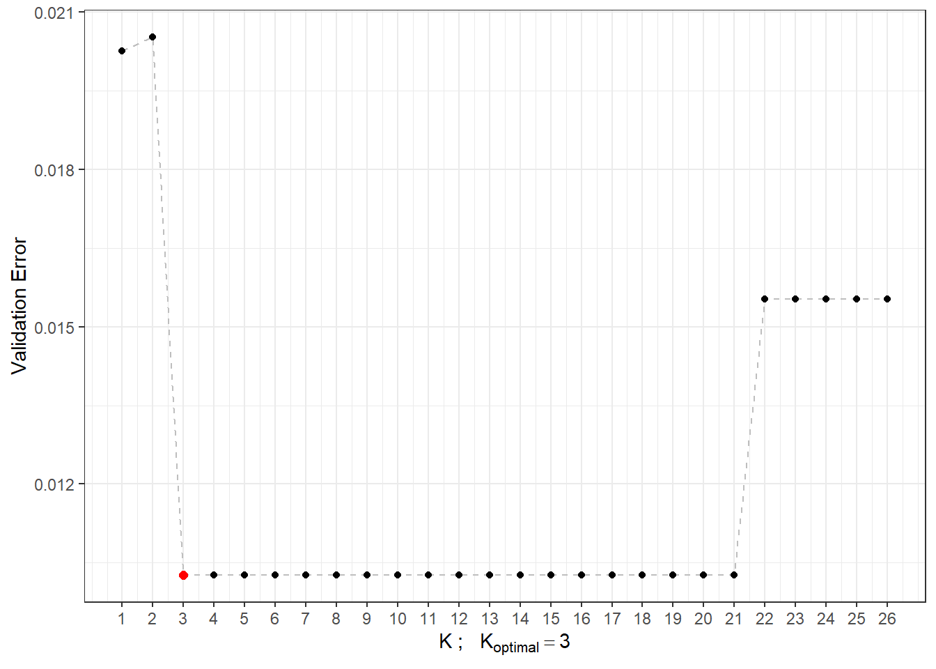

Figure 5.12: Dependency of validation error on the value of \(K\), i.e., the number of neighbors.

Now that we know the optimal value of the parameter \(K\), we can construct the final model.

Code

neighb.model <- classif.knn(group = y.train, fdataobj = x.train, knn = K.opt)

# predictions
model.neighb.predict <- predict(neighb.model, 
                                new.fdataobj = fdata(X.test))

# accuracy on test data
presnost <- table(as.numeric(factor(Y.test)), model.neighb.predict) |>
  prop.table() |>
  diag() |>
  sum()

Thus, we see that the error of the model built using the \(K\) nearest neighbors method with the optimal choice of \(K_{optimal}\) equal to 3, which we determined through cross-validation, is 0.0133 on the training data and 0.0769 on the test data.

To compare individual models, we can use both types of errors; for clarity, we will store them in a table.

Code

RESULTS <- data.frame(model = 'KNN', 
                      Err.train = 1 - neighb.model$max.prob,
                      Err.test = 1 - presnost)

6.4.2 Linear Discriminant Analysis

As a second method for constructing a classifier, we will consider Linear Discriminant Analysis (LDA). Since this method cannot be applied to functional data, we must first discretize it using functional principal component analysis. We will then perform the classification algorithm on the scores of the first \(p\) principal components. We will choose the number of components \(p\) such that the first \(p\) principal components together explain at least 90% of the variability in the data.

Let’s first perform functional principal component analysis and determine the number \(p\).

Code

# Principal component analysis
data.PCA <- pca.fd(X.train, nharm = 10) # nharm - maximum number of PCs
nharm <- which(cumsum(data.PCA$varprop) >= 0.9)[1] # determining p
if(nharm == 1) nharm <- 2 # to plot graphs, we need at least 2 PCs

data.PCA <- pca.fd(X.train, nharm = nharm) 
data.PCA.train <- as.data.frame(data.PCA$scores) # scores of the first p PCs
data.PCA.train$Y <- factor(Y.train) # membership to classes

In this specific case, we took the number of principal components to be \(p=\) 2, which together explain 93.12 \(\%\) of the variability in the data. The first principal component explains 77.7 % and the second 15.42 \(\%\) of the variability. We can visually display the scores of the first two principal components, color-coded according to classification class membership.

Code

data.PCA.train |> ggplot(aes(x = V1, y = V2, colour = Y)) +
  geom_point(size = 1.5) + 
  labs(x = paste('1st Principal Component (explained variability', 
                 round(100 * data.PCA$varprop[1], 2), '%)'),
       y = paste('2nd Principal Component (', 
                 round(100 * data.PCA$varprop[2], 2), '%)'),
       colour = 'Fat Content') +
  scale_color_discrete(labels = c("low", "high")) + 
  theme_bw()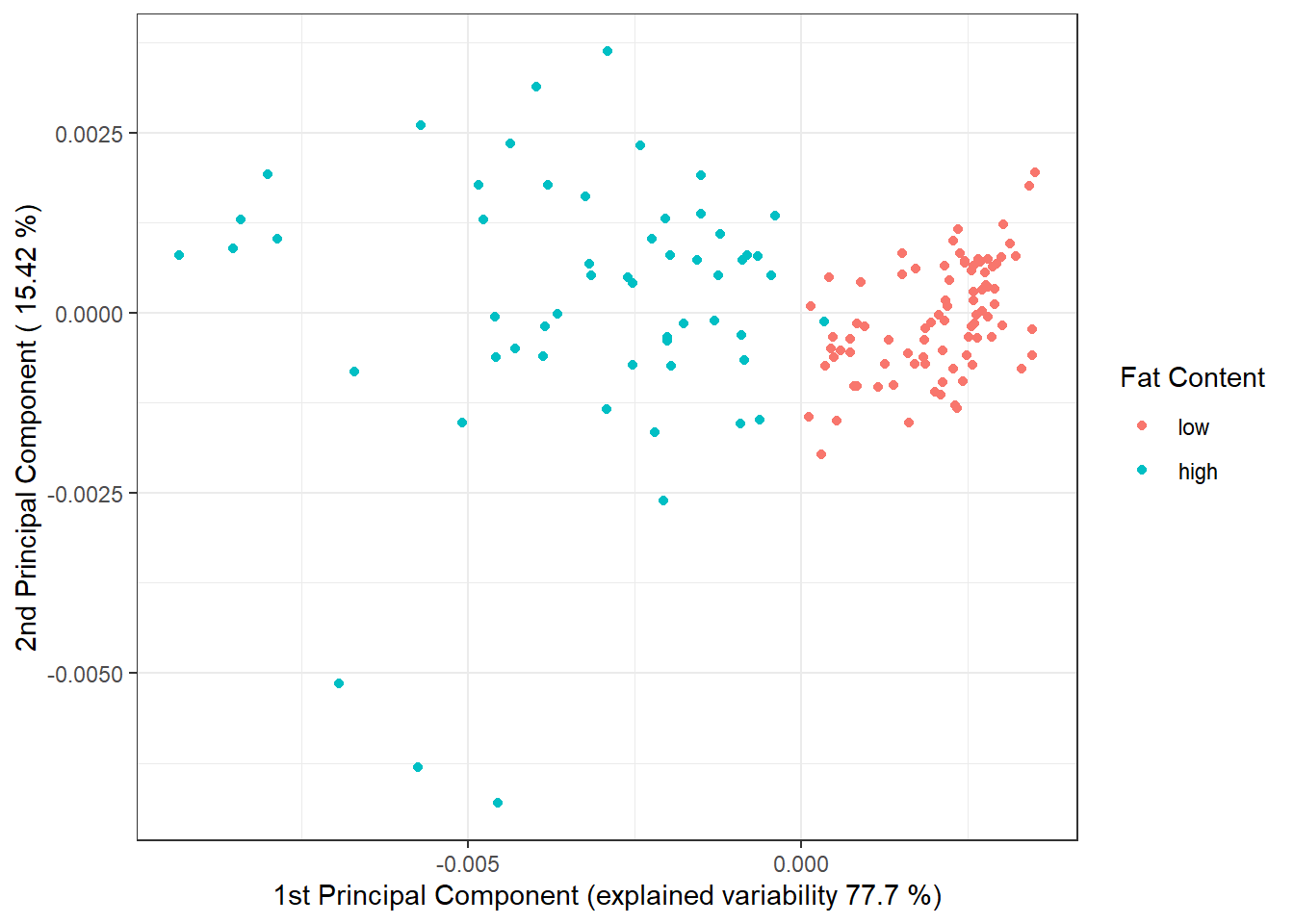

Figure 6.11: Scores of the first two principal components for training data. Points are color-coded according to classification class membership.

To determine the classification accuracy on the test data, we need to compute the scores for the first 2 principal components for the test data. These scores are calculated using the formula:

\[ \xi_{i, j} = \int \left( X_i(t) - \mu(t)\right) \cdot \rho_j(t)\text dt, \] where \(\mu(t)\) is the mean function and \(\rho_j(t)\) is the eigenfunction (functional principal component).

Code

# Calculation of scores for test functions
scores <- matrix(NA, ncol = nharm, nrow = length(Y.test)) # empty matrix

for(k in 1:dim(scores)[1]) {
  xfd = X.test[k] - data.PCA$meanfd[1] # k-th observation - mean function
  scores[k, ] = inprod(xfd, data.PCA$harmonics) 
  # scalar product of the residual and eigenfunctions rho (functional principal components)
}

data.PCA.test <- as.data.frame(scores)
data.PCA.test$Y <- factor(Y.test)
colnames(data.PCA.test) <- colnames(data.PCA.train) 

Now we can construct the classifier on the training part of the data.

Code

# model
clf.LDA <- lda(Y ~ ., data = data.PCA.train)

# accuracy on training data
predictions.train <- predict(clf.LDA, newdata = data.PCA.train)
presnost.train <- table(data.PCA.train$Y, predictions.train$class) |>
  prop.table() |> diag() |> sum()
  
# accuracy on test data
predictions.test <- predict(clf.LDA, newdata = data.PCA.test)
presnost.test <- table(data.PCA.test$Y, predictions.test$class) |>
  prop.table() |> diag() |> sum()

We have calculated the error of the classifier on the training data (4 %) as well as on the test data (9.23 %).

To visually represent the method, we can mark the decision boundary in the plot of the scores of the first two principal components. We will calculate this boundary on a dense grid of points and display it using the geom_contour() function.

Code

# Add the decision boundary
np <- 1001 # number of grid points
# x-axis ... 1st PC
nd.x <- seq(from = min(data.PCA.train$V1), 
            to = max(data.PCA.train$V1), length.out = np)
# y-axis ... 2nd PC
nd.y <- seq(from = min(data.PCA.train$V2), 
            to = max(data.PCA.train$V2), length.out = np)
# case for 2 PCs ... p = 2
nd <- expand.grid(V1 = nd.x, V2 = nd.y)
# case for p = 3
if(dim(data.PCA.train)[2] == 4) {
  nd <- expand.grid(V1 = nd.x, V2 = nd.y, V3 = data.PCA.train$V3[1])}
# case for p = 4
if(dim(data.PCA.train)[2] == 5) {
  nd <- expand.grid(V1 = nd.x, V2 = nd.y, V3 = data.PCA.train$V3[1],
                    V4 = data.PCA.train$V4[1])}
# case for p = 5
if(dim(data.PCA.train)[2] == 6) {
  nd <- expand.grid(V1 = nd.x, V2 = nd.y, V3 = data.PCA.train$V3[1],
                    V4 = data.PCA.train$V4[1], V5 = data.PCA.train$V5[1])}

# Add Y = 0, 1
nd <- nd |> mutate(prd = as.numeric(predict(clf.LDA, newdata = nd)$class))

data.PCA.train |> ggplot(aes(x = V1, y = V2, colour = Y)) +
  geom_point(size = 1.5) + 
  labs(x = paste('1st Principal Component (explained variability', 
                 round(100 * data.PCA$varprop[1], 2), '%)'),
       y = paste('2nd Principal Component (', 
                 round(100 * data.PCA$varprop[2], 2), '%)'),
       colour = 'Fat Content') +
  scale_color_discrete(labels = c("low", "high")) + 
  theme_bw() +
  geom_contour(data = nd, aes(x = V1, y = V2, z = prd), colour = 'black')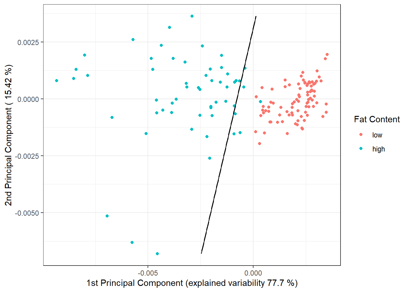

Figure 6.12: Scores of the first two principal components, color-coded according to classification class. The decision boundary (a line in the plane of the first two principal components) between classes constructed using LDA is marked in black.

We see that the decision boundary is a line, a linear function in the 2D space, which is what we expected from LDA. Finally, we will add the errors to the summary table.

Code

Res <- data.frame(model = 'LDA', 
                  Err.train = 1 - presnost.train,
                  Err.test = 1 - presnost.test)

RESULTS <- rbind(RESULTS, Res)

6.4.3 Quadratic Discriminant Analysis

Next, let’s build a classifier using Quadratic Discriminant Analysis (QDA). This is analogous to LDA, with the difference that we now allow for different covariance matrices for each class of the normal distribution from which the corresponding scores originate. This dropped assumption of equal covariance matrices leads to a quadratic boundary between the classes.

In R, QDA is performed similarly to LDA in the previous section. We would again calculate scores for the training and test functions using functional principal component analysis and construct a classifier based on the scores of the first \(p\) principal components to predict the membership of the test curves to class \(Y^* \in \{0, 1\}\).

However, we do not need to perform functional PCA, as we can use the results from the LDA section.

Thus, we can directly proceed to constructing the classifier using the qda() function. Subsequently, we will calculate the accuracy of the classifier on the test and training data.

Code

# model
clf.QDA <- qda(Y ~ ., data = data.PCA.train)

# accuracy on training data
predictions.train <- predict(clf.QDA, newdata = data.PCA.train)
presnost.train <- table(data.PCA.train$Y, predictions.train$class) |>
  prop.table() |> diag() |> sum()
  
# accuracy on test data
predictions.test <- predict(clf.QDA, newdata = data.PCA.test)
presnost.test <- table(data.PCA.test$Y, predictions.test$class) |>
  prop.table() |> diag() |> sum()

We have thus calculated the error of the classifier on the training data (0.67 %) as well as on the test data (1.54 %).

To visually represent the method, we can mark the decision boundary in the plot of the scores of the first two principal components. We will calculate this boundary on a dense grid of points and display it using the geom_contour() function, just as we did in the case of LDA.

Code

nd <- nd |> mutate(prd = as.numeric(predict(clf.QDA, newdata = nd)$class))

data.PCA.train |> ggplot(aes(x = V1, y = V2, colour = Y)) +
  geom_point(size = 1.5) + 
  labs(x = paste('1st Principal Component (explained variability', 
                 round(100 * data.PCA$varprop[1], 2), '%)'),
       y = paste('2nd Principal Component (', 
                 round(100 * data.PCA$varprop[2], 2), '%)'),
       colour = 'Fat Content') +
  scale_color_discrete(labels = c("low", "high")) + 
  theme_bw() +
  geom_contour(data = nd, aes(x = V1, y = V2, z = prd), colour = 'black')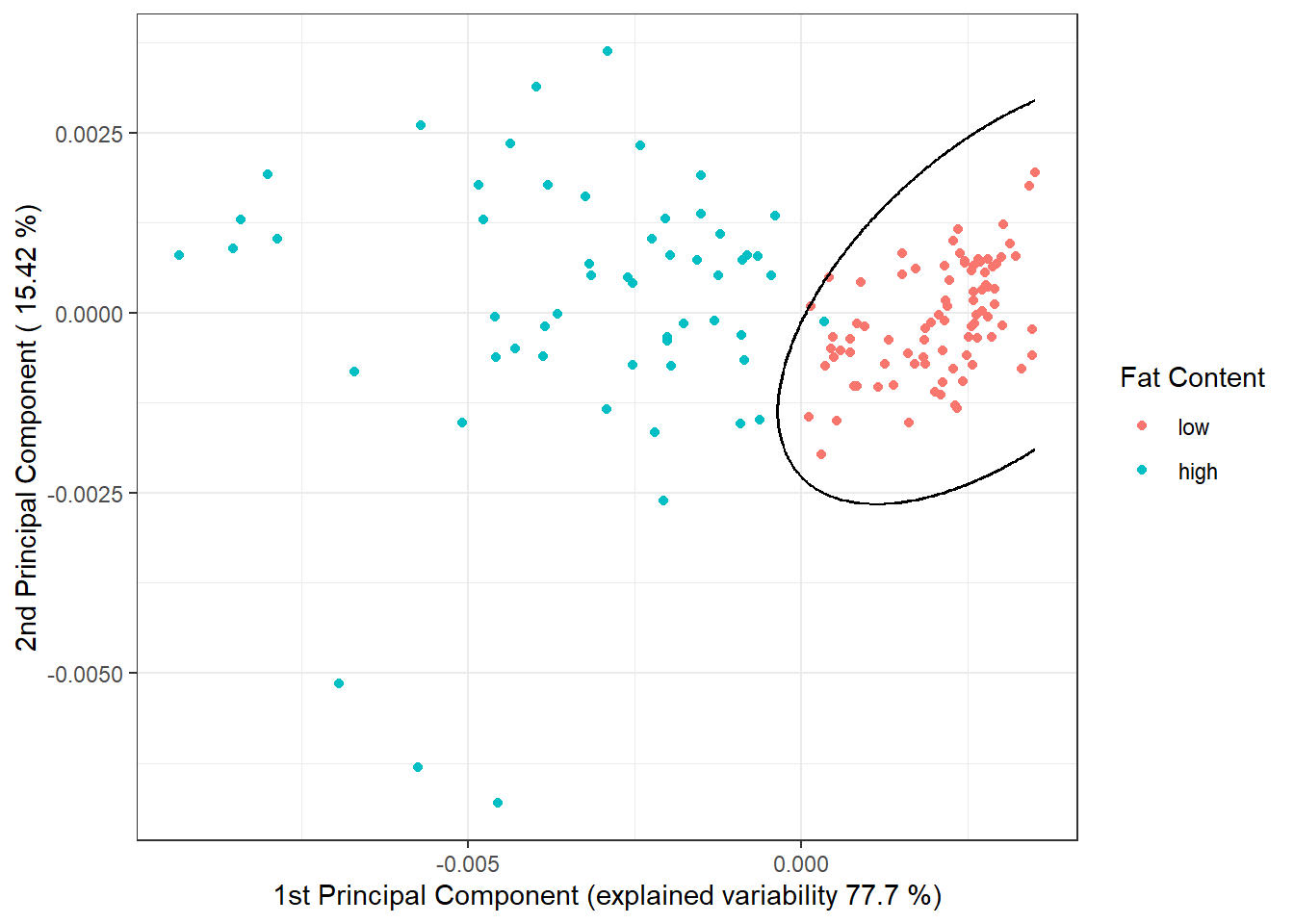

Figure 1.26: Scores of the first two principal components, color-coded according to class. The decision boundary (a parabola in the plane of the first two principal components) between classes constructed using QDA is marked in black.

Note that the decision boundary between the classification classes is now a parabola, which only (at least visually) differs very little from a line.

Finally, we will add the errors to the summary table.

Code

Res <- data.frame(model = 'QDA', 
                  Err.train = 1 - presnost.train,
                  Err.test = 1 - presnost.test)

RESULTS <- rbind(RESULTS, Res)

6.4.4 Logistic Regression

Logistic regression can be performed in two ways. First, we can use the functional analogue of classical logistic regression, and second, we can perform classical multivariate logistic regression on the scores of the first \(p\) principal components.

6.4.4.1 Functional Logistic Regression

Similarly to the finite-dimensional case of input data, we consider a logistic model in the form:

\[ g\left(\mathbb E [Y|X = x]\right) = \eta (x) = g(\pi(x)) = \alpha + \int \beta(t)\cdot x(t) \text d t, \] where \(\eta(x)\) is the linear predictor taking values from the interval \((-\infty, \infty)\), \(g(\cdot)\) is the link function (in the case of logistic regression, this is the logit function \(g: (0,1) \rightarrow \mathbb R,\ g(p) = \ln\frac{p}{1-p}\)), and \(\pi(x)\) is the conditional probability

\[ \pi(x) = \text{Pr}(Y = 1 | X = x) = g^{-1}(\eta(x)) = \frac{\text e^{\alpha + \int \beta(t)\cdot x(t) \text d t}}{1 + \text e^{\alpha + \int \beta(t)\cdot x(t) \text d t}}, \]

where \(\alpha\) is a constant and \(\beta(t) \in L^2[a, b]\) is a parameter function. Our goal is to estimate this parameter function.

For functional logistic regression, we will use the fregre.glm() function from the fda.usc package. First, we will create suitable objects for constructing the classifier.

Code

# create suitable objects
x.train <- fdata(X.train)
y.train <- as.numeric(Y.train) 

# points where the functions are evaluated
tt <- x.train[["argvals"]]

dataf <- as.data.frame(y.train) 
colnames(dataf) <- "Y"

nbasis.x <- 100

# B-spline basis 
basis1 <- create.bspline.basis(rangeval = range(tt), norder = 4, nbasis = nbasis.x)

To estimate the parameter function \(\beta(t)\), we need to express it in some basis representation, in this case, the B-spline basis. However, we need to find a suitable number of basis functions. We could determine this based on the error on the training data, but this data would tend to favor selecting a large number of bases, leading to overfitting the model.

Let’s illustrate this with the following case. For each number of bases \(n_{basis} \in \{4, 5, \dots, 30\}\), we will train a model on the training data, determine the error rate on it, and also calculate the error rate on the test data. Remember that we cannot use the same data for selecting the appropriate number of bases when estimating the test error, as this would underestimate the error.

Code

n.basis.max <- 30
n.basis <- 4:n.basis.max
pred.baz <- matrix(NA, nrow = length(n.basis), ncol = 2, 
                   dimnames = list(n.basis, c('Err.train', 'Err.test')))

for (i in n.basis) {
  # bases for betas
  basis2 <- create.bspline.basis(rangeval = range(tt), nbasis = i)
  # relationship
  f <- Y ~ x
  # bases for x and betas
  basis.x <- list("x" = basis1) # smoothed data
  basis.b <- list("x" = basis2)
  # input data for the model
  ldata <- list("df" = dataf, "x" = x.train)
  # binomial model ... logistic regression model
  model.glm <- fregre.glm(f, family = binomial(), data = ldata,
                          basis.x = basis.x, basis.b = basis.b)
  
  # accuracy on training data
  predictions.train <- predict(model.glm, newx = ldata)
  predictions.train <- data.frame(Y.pred = ifelse(predictions.train < 1/2, 0, 1))
  presnost.train <- table(Y.train, predictions.train$Y.pred) |>
    prop.table() |> diag() |> sum()
    
  # accuracy on test data
  newldata = list("df" = as.data.frame(Y.test), "x" = fdata(X.test))
  predictions.test <- predict(model.glm, newx = newldata)
  predictions.test <- data.frame(Y.pred = ifelse(predictions.test < 1/2, 0, 1))
  presnost.test <- table(Y.test, predictions.test$Y.pred) |>
    prop.table() |> diag() |> sum()
  
  # insert into matrix
  pred.baz[as.character(i), ] <- 1 - c(presnost.train, presnost.test)
} 

pred.baz <- as.data.frame(pred.baz)
pred.baz$n.basis <- n.basis

Let’s visualize the progression of both types of errors in a graph depending on the number of basis functions.

Code

n.basis.beta.opt <- pred.baz$n.basis[which.min(pred.baz$Err.test)]

pred.baz |> ggplot(aes(x = n.basis, y = Err.test)) + 
  geom_line(linetype = 'dashed', colour = 'black') + 
  geom_line(aes(x = n.basis, y = Err.train), colour = 'deepskyblue3', 
            linetype = 'dashed', linewidth = 0.5) + 
  geom_point(size = 1.5) + 
  geom_point(aes(x = n.basis, y = Err.train), colour = 'deepskyblue3', 
             size = 1.5) + 
  geom_point(aes(x = n.basis.beta.opt, y = min(pred.baz$Err.test)),
             colour = 'red', size = 2) +
  theme_bw() + 
  labs(x = bquote(paste(n[basis], ' ;   ', 
                        n[optimal] == .(n.basis.beta.opt))),
        y = 'Error Rate')

## Warning: Use of `pred.baz$Err.test` is discouraged.
## ℹ Use `Err.test` instead.

## Warning in geom_point(aes(x = n.basis.beta.opt, y = min(pred.baz$Err.test)), : All aesthetics have length 1, but the data has 27 rows.
## ℹ Please consider using `annotate()` or provide this layer with data containing
##   a single row.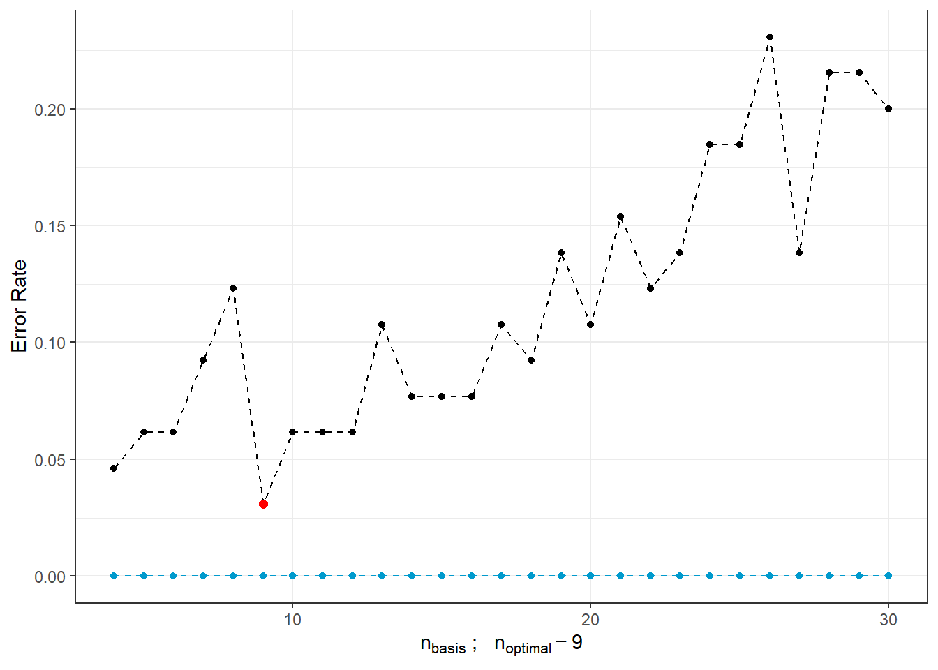

Figure 5.16: Dependence of test and training error rates on the number of basis functions for \(\beta\). The red dot represents the optimal number \(n_{optimal}\) chosen as the minimum of the test error rate, the black line represents the test error, and the blue dashed line represents the training error rate.

We see that as the number of bases for \(\beta(t)\) increases, the training error rate (blue line) tends to decrease, suggesting that we would choose large values for \(n_{basis}\) based on it. Conversely, the optimal choice based on the test error rate is \(n\) equal to 9, which is significantly smaller than 30. On the other hand, as \(n\) increases, the test error rate rises, indicating model overfitting.

For these reasons, we will use 10-fold cross-validation to determine the optimal number of basis functions for \(\beta(t)\). We take a maximum of 25 considered basis functions since, as we saw above, beyond this value, model overfitting occurs.

Code

### 10-fold cross-validation
n.basis.max <- 25
n.basis <- 4:n.basis.max
k_cv <- 10 # k-fold CV
# divide training data into k parts
folds <- createMultiFolds(X.train$fdnames$reps, k = k_cv, time = 1)
## elements that do not change during the loop
# points at which the functions are evaluated
tt <- x.train[["argvals"]]
rangeval <- range(tt)
# B-spline bases 
basis1 <- create.bspline.basis(rangeval = range(tt), nbasis = nbasis.x)
# relationship
f <- Y ~ x
# bases for x
basis.x <- list("x" = basis1)
# empty matrix to insert individual results
# columns will hold accuracy values for each part of the training set
# rows will hold values for a given number of bases
CV.results <- matrix(NA, nrow = length(n.basis), ncol = k_cv, 
                     dimnames = list(n.basis, 1:k_cv))

Now we have everything prepared to calculate the error rate on each of the ten subsets of the training set. We will then determine the average and take the optimal \(n\) as the argument of the minimum validation error rate.

Code

for (index in 1:k_cv) {
  # define the given index set
  fold <- folds[[index]]
    
  x.train.cv <- subset(X.train, c(1:length(X.train$fdnames$reps)) %in% fold) |>
    fdata()
  y.train.cv <- subset(Y.train, c(1:length(X.train$fdnames$reps)) %in% fold) |>
    as.numeric()
  
  x.test.cv <- subset(X.train, !c(1:length(X.train$fdnames$reps)) %in% fold) |>
    fdata()
  y.test.cv <- subset(Y.train, !c(1:length(X.train$fdnames$reps)) %in% fold) |>
    as.numeric()
  
  dataf <- as.data.frame(y.train.cv) 
  colnames(dataf) <- "Y"
  
  for (i in n.basis) {
    # bases for betas
    basis2 <- create.bspline.basis(rangeval = rangeval, nbasis = i)
    
    basis.b <- list("x" = basis2)
    # input data for the model
    ldata <- list("df" = dataf, "x" = x.train.cv)
    # binomial model ... logistic regression model
    model.glm <- fregre.glm(f, family = binomial(), data = ldata,
                            basis.x = basis.x, basis.b = basis.b)
    
    # accuracy on the validation part 
    newldata = list("df" = as.data.frame(y.test.cv), "x" = x.test.cv)
    predictions.valid <- predict(model.glm, newx = newldata)
    predictions.valid <- data.frame(Y.pred = ifelse(predictions.valid < 1/2, 0, 1))
    presnost.valid <- table(y.test.cv, predictions.valid$Y.pred) |>
      prop.table() |> diag() |> sum()
    
    # insert into the matrix
    CV.results[as.character(i), as.character(index)] <- presnost.valid
  } 
}

# calculate average accuracy for each n across folds
CV.results <- apply(CV.results, 1, mean)
n.basis.opt <- n.basis[which.max(CV.results)]
presnost.opt.cv <- max(CV.results)

Let’s plot the course of validation error with the highlighted optimal value of \(n_{optimal}\) equal to 16 and validation error equal to 0.0483.

Code

CV.results <- data.frame(n.basis = n.basis, CV = CV.results)
CV.results |> ggplot(aes(x = n.basis, y = 1 - CV)) + 
  geom_line(linetype = 'dashed', colour = 'grey') + 
  geom_point(size = 1.5) + 
  geom_point(aes(x = n.basis.opt, y = 1 - presnost.opt.cv), colour = 'red', size = 2) +
  theme_bw() + 
  labs(x = bquote(paste(n[basis], ' ;   ', 
                        n[optimal] == .(n.basis.opt))),
       y = 'Validation Error') + 
  scale_x_continuous(breaks = n.basis) + 
  theme(panel.grid.minor = element_blank())

## Warning in geom_point(aes(x = n.basis.opt, y = 1 - presnost.opt.cv), colour = "red", : All aesthetics have length 1, but the data has 22 rows.
## ℹ Please consider using `annotate()` or provide this layer with data containing
##   a single row.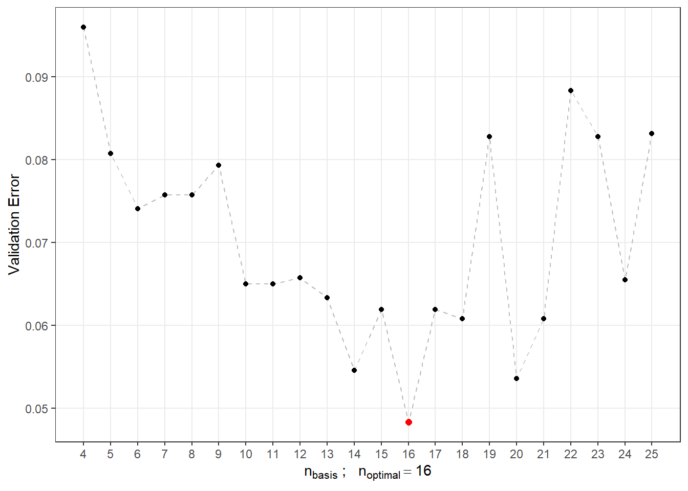

Figure 5.17: Dependence of validation error on the value of \(n_{basis}\), that is, the number of bases.

Now we can define the final model using functional logistic regression, choosing a B-spline basis for \(\beta(t)\) with 16 bases.

Code

# optimal model
basis2 <- create.bspline.basis(rangeval = range(tt), nbasis = n.basis.opt)
f <- Y ~ x
# bases for x and betas
basis.x <- list("x" = basis1) 
basis.b <- list("x" = basis2)
# input data for the model
dataf <- as.data.frame(y.train) 
colnames(dataf) <- "Y"
ldata <- list("df" = dataf, "x" = x.train)
# binomial model ... logistic regression model
model.glm <- fregre.glm(f, family = binomial(), data = ldata,
                        basis.x = basis.x, basis.b = basis.b,
                        maxit = 1000, epsilon = 1e-2)

# accuracy on the training data
predictions.train <- predict(model.glm, newx = ldata)
predictions.train <- data.frame(Y.pred = ifelse(predictions.train < 1/2, 0, 1))
presnost.train <- table(Y.train, predictions.train$Y.pred) |>
  prop.table() |> diag() |> sum()
  
# accuracy on the test data
newldata = list("df" = as.data.frame(Y.test), "x" = fdata(X.test))
predictions.test <- predict(model.glm, newx = newldata)
predictions.test <- data.frame(Y.pred = ifelse(predictions.test < 1/2, 0, 1))
presnost.test <- table(Y.test, predictions.test$Y.pred) |>
  prop.table() |> diag() |> sum()

We have calculated the training error (equal to 0 %) and the test error (equal to 7.69 %). For better understanding, we can also plot the values of the estimated probabilities of belonging to the classification class \(Y = 1\) on the training data in relation to the values of the linear predictor.

Code

data.frame(
  linear.predictor = model.glm$linear.predictors,
  response = model.glm$fitted.values,
  Y = factor(y.train)
) |> ggplot(aes(x = linear.predictor, y = response, colour = Y)) + 
  geom_point(size = 1.5) + 
  scale_color_discrete(labels = c("small", "large")) + 
  geom_abline(aes(slope = 0, intercept = 0.5), linetype = 'dashed') + 
  theme_bw() + 
  labs(x = 'Linear Predictor',
       y = 'Estimated Probabilities Pr(Y = 1|X = x)',
       colour = 'Fat Content')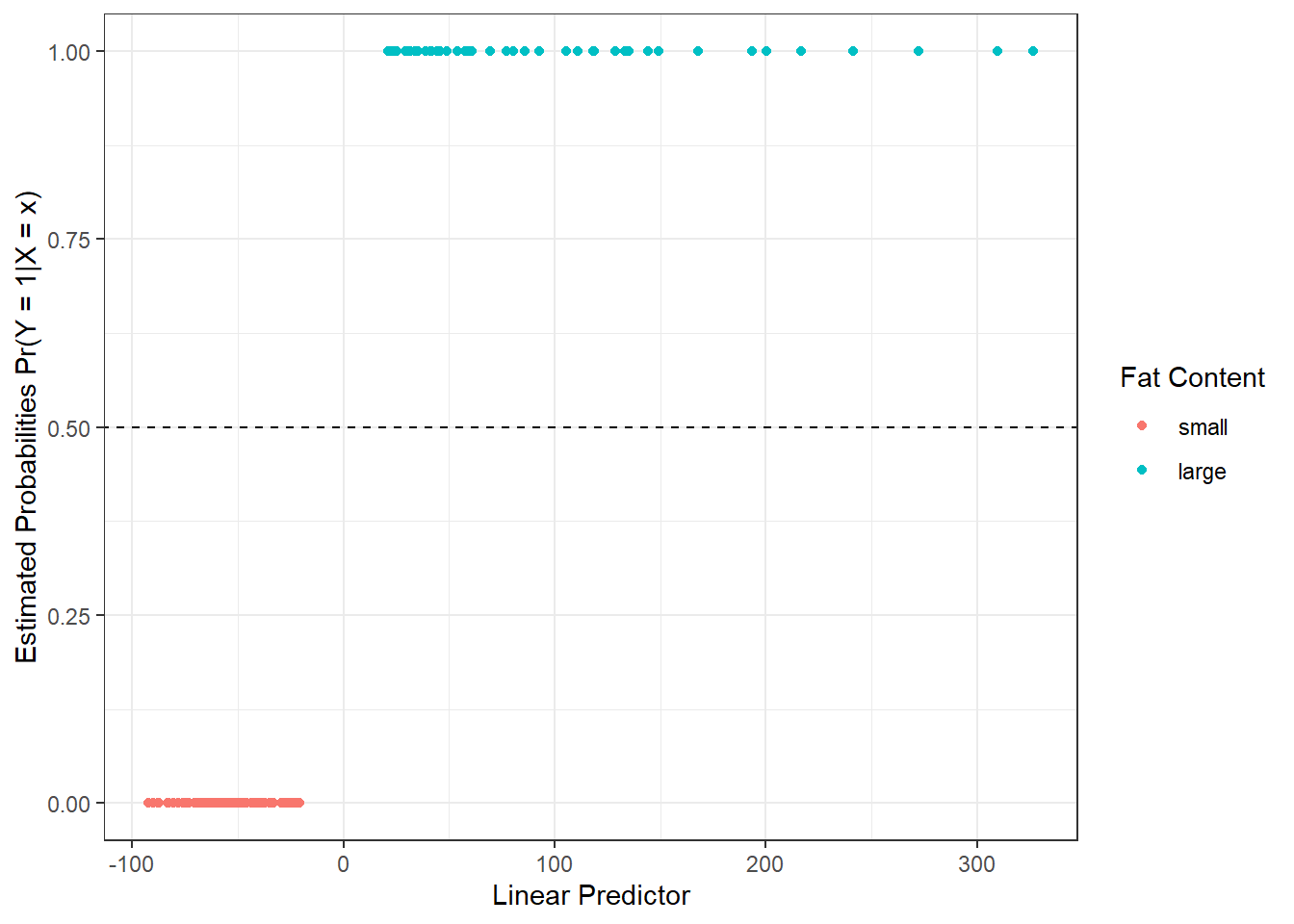 

Figure 6.13: Dependence of estimated probabilities on the values of the linear predictor. Points are colored according to their belonging to the classification class.

We can also display the course of the estimated parametric function \(\beta(t)\) for reference.

Code

t.seq <- seq(min(t), max(t), length = 1001)
beta.seq <- eval.fd(evalarg = t.seq, fdobj = model.glm$beta.l$x)

data.frame(t = t.seq, beta = beta.seq) |> 
  ggplot(aes(t, beta)) + 
  geom_abline(aes(slope = 0, intercept = 0), linetype = 'dashed', 
              linewidth = 0.5, colour = 'grey') +
  geom_line() + 
  theme_bw() +
  labs(x = expression(x[1]),
       y = expression(widehat(beta)(t))) + 
  theme(panel.grid.major = element_blank(),
        panel.grid.minor = element_blank())

Figure 5.18: Course of the estimate of the parametric function \(\beta(t), t \in [850, 1050]\).

We see that the values of the function \(\hat\beta(t)\) stay around zero for times \(t\) from the middle and beginning of the interval \([850, 1050]\), while for later times, the values are higher. This implies the differences between functions from the classification classes at the beginning and end of the interval, while in the middle of the interval, the functions are very similar.

We will again add the results to the summary table.

Code

Res <- data.frame(model = 'LR functional', 
                  Err.train = 1 - presnost.train,
                  Err.test = 1 - presnost.test)

RESULTS <- rbind(RESULTS, Res)

6.4.4.2 Logistic Regression with Principal Component Analysis

To construct this classifier, we need to perform functional principal component analysis, determine the appropriate number of components, and compute score values for the test data. We have already done this in the linear discriminant analysis section, so we will use these results in the following part.

We can now construct the logistic regression model using the glm(, family = binomial) function.

Code

# model
clf.LR <- glm(Y ~  ., data = data.PCA.train, family = binomial)

## Warning: glm.fit: fitted probabilities numerically 0 or 1 occurred

Code

# accuracy on training data
predictions.train <- predict(clf.LR, newdata = data.PCA.train, type = 'response')
predictions.train <- ifelse(predictions.train > 0.5, 1, 0)
accuracy.train <- table(data.PCA.train$Y, predictions.train) |>
  prop.table() |> diag() |> sum()
  
# accuracy on test data
predictions.test <- predict(clf.LR, newdata = data.PCA.test, type = 'response')
predictions.test <- ifelse(predictions.test > 0.5, 1, 0)
accuracy.test <- table(data.PCA.test$Y, predictions.test) |>
  prop.table() |> diag() |> sum()

We have thus calculated the error rate of the classifier on the training (0.67 %) and test data (4.62 %).

For a graphical representation of the method, we can mark the decision boundary in the plot of the scores of the first two principal components. We will calculate this boundary on a dense grid of points and display it using the geom_contour() function, just as we did for LDA and QDA.

Code

nd <- nd |> mutate(prd = as.numeric(predict(clf.LR, newdata = nd,
                                            type = 'response')))
nd$prd <- ifelse(nd$prd > 0.5, 1, 0)

data.PCA.train |> ggplot(aes(x = V1, y = V2, colour = Y)) +
  geom_point(size = 1.5) + 
  labs(x = paste('1st principal component (explained variance', 
                 round(100 * data.PCA$varprop[1], 2), '%)'),
       y = paste('2nd principal component (', 
                 round(100 * data.PCA$varprop[2], 2), '%)'),
       colour = 'Fat content') +
  scale_colour_discrete(labels = c("low", "high")) +
  theme_bw() +
  geom_contour(data = nd, aes(x = V1, y = V2, z = prd), colour = 'black')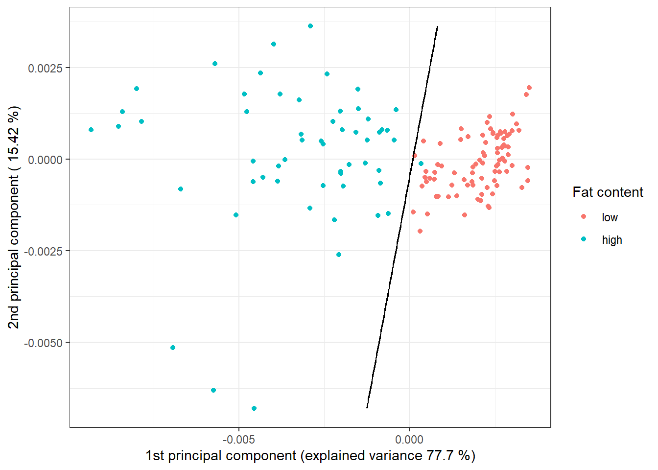

Figure 1.28: Scores of the first two principal components, color-coded according to class membership. The decision boundary (a line in the plane of the first two principal components) between the classes is marked in black and constructed using logistic regression.

Note that the decision boundary between the classification classes is now a line, as in the case of LDA.

Finally, let’s add the error rates to the summary table.

Code

Res <- data.frame(model = 'LR score', 
                  Err.train = 1 - accuracy.train,
                  Err.test = 1 - accuracy.test)

RESULTS <- rbind(RESULTS, Res)

6.4.5 Decision Trees

In this section, we will look at a very different approach to constructing a classifier than methods like LDA or logistic regression. Decision trees are a very popular tool for classification, but as with some previous methods, they are not directly designed for functional data. However, there are ways to convert functional objects into multidimensional ones and then apply the decision tree algorithm to them. We can consider the following approaches:

• An algorithm constructed on the basis of coefficients,
• Using principal component scores,
• Applying discretization of the interval and evaluating the function only on a finite grid of points.

We will first focus on interval discretization and then compare the results with the remaining two approaches to constructing a decision tree.

6.4.5.1 Interval Discretization

First, we need to define the points from the interval \(I = [850, 1050]\) at which we will evaluate the functions. Next, we will create an object in which the rows represent individual (discretized) functions and the columns represent time points. Finally, we will append the column \(Y\) with information about class membership, and we will repeat the same for the test data.

Code

# sequence of points at which we will evaluate the functions
t.seq <- seq(min(t), max(t), length = 101)
   
grid.data <- eval.fd(fdobj = X.train, evalarg = t.seq)
grid.data <- as.data.frame(t(grid.data)) # transpose for functions in rows
grid.data$Y <- Y.train |> factor()

grid.data.test <- eval.fd(fdobj = X.test, evalarg = t.seq)
grid.data.test <- as.data.frame(t(grid.data.test))
grid.data.test$Y <- Y.test |> factor()

Now we can construct a decision tree where all time points from the vector t.seq will serve as predictors. This classification method is not susceptible to multicollinearity, so we do not need to worry about it. We will choose accuracy as the metric.

Code

# constructing the model
clf.tree <- train(Y ~ ., data = grid.data, 
                 method = "rpart", 
                 trControl = trainControl(method = "CV", number = 10),
                 metric = "Accuracy")

# accuracy on training data
predictions.train <- predict(clf.tree, newdata = grid.data)
accuracy.train <- table(Y.train, predictions.train) |>
  prop.table() |> diag() |> sum()
  
# accuracy on test data
predictions.test <- predict(clf.tree, newdata = grid.data.test)
accuracy.test <- table(Y.test, predictions.test) |>
  prop.table() |> diag() |> sum()

Thus, the error rate of the classifier on the test data is 1.54 % and on the training data is 0.67 %.

Graphically, we can visualize the decision tree using the fancyRpartPlot() function. We will set the node colors to reflect the previous color coding. This will be an unpruned tree.

Code

colnames(grid.data) <- c(paste0('time:', t.seq), 'Y')
fancyRpartPlot(rpart(Y ~ ., data = grid.data, method = "class"),
               sub = '', palettes = c('Reds', 'Blues')) 

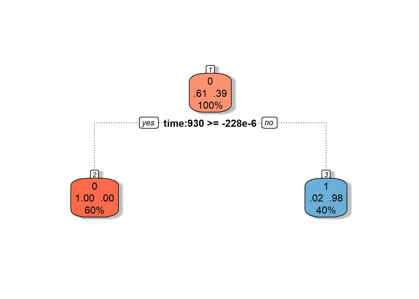
Figure 1.30: Graphical representation of the unpruned decision tree. Nodes belonging to class 1 are colored in shades of blue, and nodes belonging to class 0 are colored in shades of red.

We can also visualize the final pruned decision tree.

Code

rpart.plot::rpart.plot(clf.tree$finalModel, # final model ... pruned tree
                       extra = 104, # display of desired information
                       box.palette = c('Reds', 'Blues'),
                       branch.lty = 3, # dotted branch lines
                       shadow.col = 0, # shadows under the node boxes
                       nn = FALSE, 
                       under = FALSE, 
                       digits = 2)

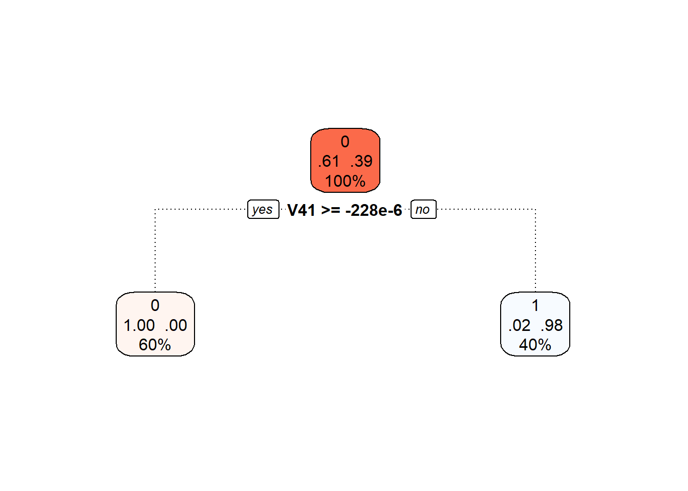
Figure 6.14: Final pruned decision tree.

Finally, let’s add the training and test error rates to the summary table.

Code

Res <- data.frame(model = 'Tree - discretization', 
                  Err.train = 1 - accuracy.train,
                  Err.test = 1 - accuracy.test)

RESULTS <- rbind(RESULTS, Res)

6.4.5.2 Principal Component Scores

Another option for constructing a decision tree is to use principal component scores. Since we have already computed the scores for previous classification methods, we will utilize this knowledge and build a decision tree based on the scores of the first 2 principal components.

Code

# constructing the model
clf.tree.PCA <- train(Y ~ ., data = data.PCA.train, 
                 method = "rpart", 
                 trControl = trainControl(method = "CV", number = 10),
                 metric = "Accuracy")

# accuracy on training data
predictions.train <- predict(clf.tree.PCA, newdata = data.PCA.train)
accuracy.train <- table(Y.train, predictions.train) |>
  prop.table() |> diag() |> sum()
  
# accuracy on test data
predictions.test <- predict(clf.tree.PCA, newdata = data.PCA.test)
accuracy.test <- table(Y.test, predictions.test) |>
  prop.table() |> diag() |> sum()

Thus, the error rate of the decision tree on the test data is 6.15 % and on the training data is 0.67 %.

We can visualize the decision tree constructed on the principal component scores using the fancyRpartPlot() function. We will set the node colors to reflect the previous color coding. This will be an unpruned tree.

Code

fancyRpartPlot(rpart(Y ~ ., data = data.PCA.train, method = "class"),
               sub = '', palettes = c('Reds', 'Blues')) 

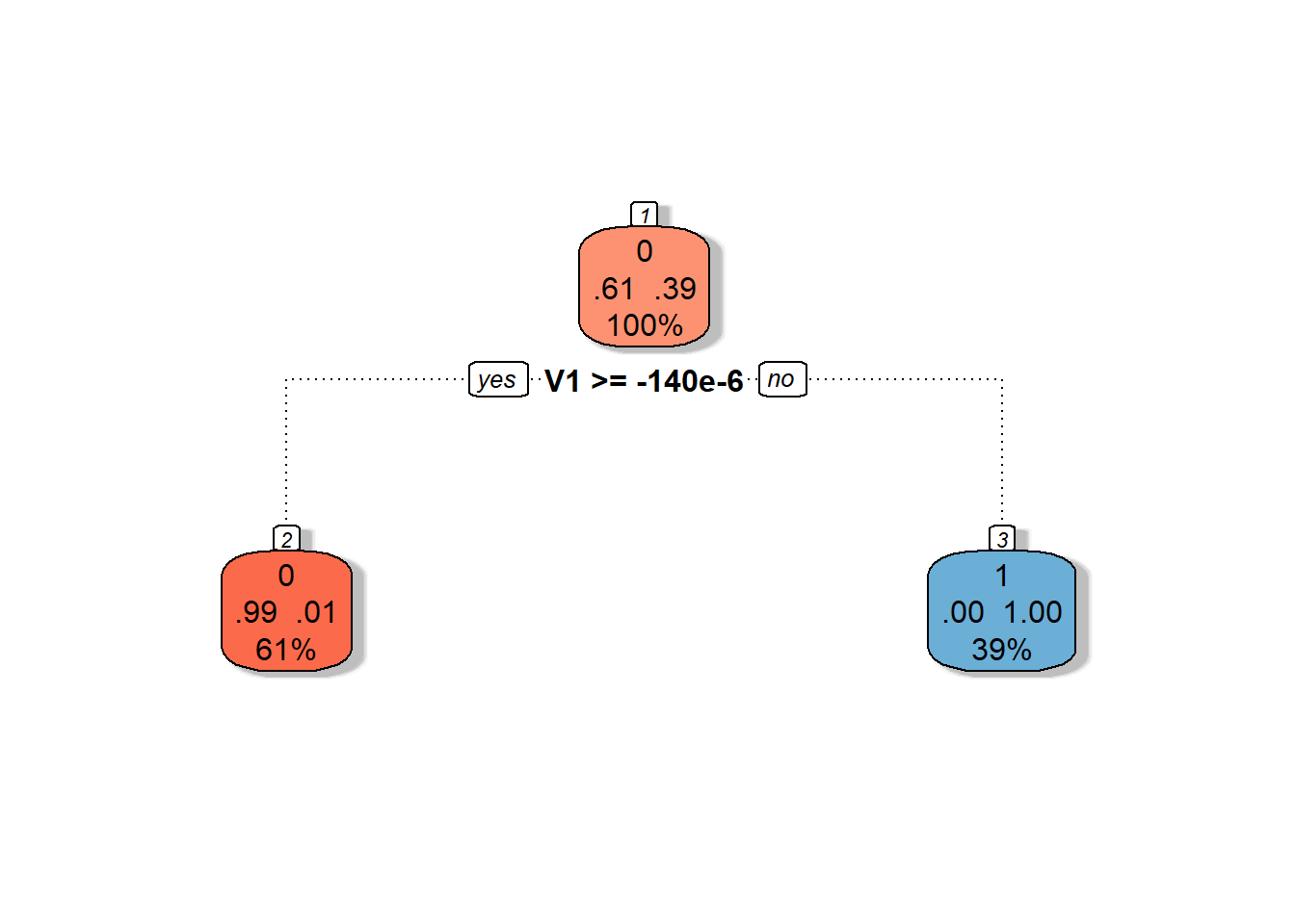
Figure 1.32: Graphical representation of the unpruned decision tree constructed on principal component scores. Nodes belonging to class 1 are colored in shades of blue, and nodes belonging to class 0 are colored in shades of red.

We can also visualize the final pruned decision tree.

Code

rpart.plot::rpart.plot(clf.tree.PCA$finalModel, # final model 
                       extra = 104, # display of desired information
                       box.palette = c('Reds', 'Blues'),
                       branch.lty = 3, # dotted branch lines
                       shadow.col = 0, # shadows under the node boxes
                       nn = FALSE, under = FALSE, digits = 2)

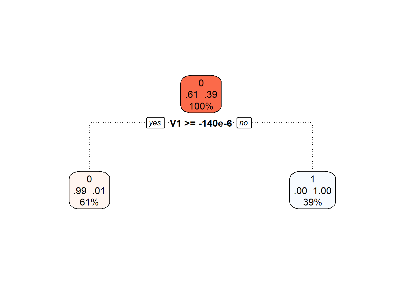
Figure 5.23: Final pruned decision tree.

Finally, let’s add the training and test error rates to the summary table.

Code

Res <- data.frame(model = 'Tree - score', 
                  Err.train = 1 - accuracy.train,
                  Err.test = 1 - accuracy.test)

RESULTS <- rbind(RESULTS, Res)

6.4.5.3 B-spline Coefficients

The last option we will use for constructing the decision tree is to utilize the coefficients expressed in the B-spline basis.

First, let’s define the necessary datasets with the coefficients.

Code

# training dataset
data.Bbasis.train <- t(X.train$coefs) |> as.data.frame()
data.Bbasis.train$Y <- factor(Y.train)

# testing dataset
data.Bbasis.test <- t(X.test$coefs) |> as.data.frame()
data.Bbasis.test$Y <- factor(Y.test)

Now we can build the classifier.

Code

# constructing the model
clf.tree.Bbasis <- train(Y ~ ., data = data.Bbasis.train, 
                 method = "rpart", 
                 trControl = trainControl(method = "CV", number = 10),
                 metric = "Accuracy")

# accuracy on training data
predictions.train <- predict(clf.tree.Bbasis, newdata = data.Bbasis.train)
accuracy.train <- table(Y.train, predictions.train) |>
  prop.table() |> diag() |> sum()
  
# accuracy on test data
predictions.test <- predict(clf.tree.Bbasis, newdata = data.Bbasis.test)
accuracy.test <- table(Y.test, predictions.test) |>
  prop.table() |> diag() |> sum()

Thus, the error rate of the decision tree on the training data is 0.67 % and on the test data is 1.54 %.

We can visualize the decision tree constructed on the B-spline coefficients using the fancyRpartPlot() function. We will set the node colors to reflect the previous color coding. This will be an unpruned tree.

Code

fancyRpartPlot(rpart(Y ~ ., data = data.Bbasis.train, method = "class"),
               sub = '', palettes = c('Reds', 'Blues')) 

Figure 5.24: Graphical representation of the unpruned decision tree constructed on B-spline coefficients. Nodes belonging to class 1 are colored in shades of blue, and nodes belonging to class 0 are colored in shades of red.

We can also visualize the final pruned decision tree.

Code

rpart.plot::rpart.plot(clf.tree.Bbasis$finalModel, # final model 
                       extra = 104, # display of desired information
                       box.palette = c('Reds', 'Blues'),
                       branch.lty = 3, # dotted branch lines
                       shadow.col = 0, # shadows under the node boxes
                       nn = FALSE, under = FALSE, digits = 2)

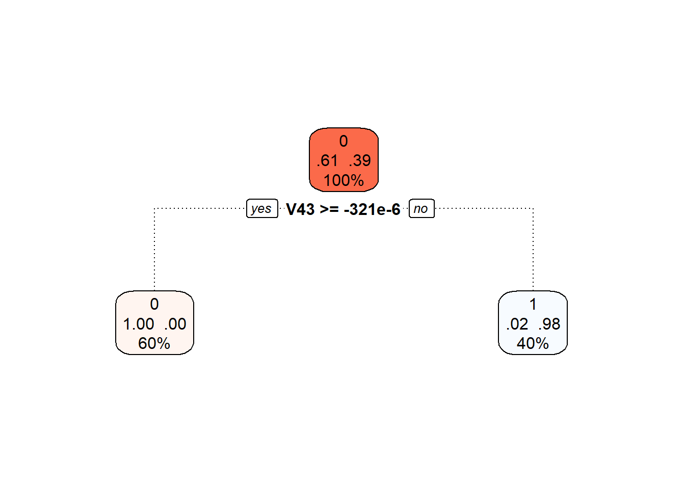
Figure 6.15: Final pruned decision tree.

Finally, let’s add the training and test error rates to the summary table.

Code

Res <- data.frame(model = 'Tree - Bbasis', 
                  Err.train = 1 - accuracy.train,
                  Err.test = 1 - accuracy.test)

RESULTS <- rbind(RESULTS, Res)

6.4.6 Random Forests

A classifier built using the random forest method involves constructing several individual decision trees, which are then combined to create a single classifier through “voting.”

Just as with decision trees, we have several options regarding which data (finite-dimensional) to use for constructing the model. We will again consider the three approaches discussed earlier. The data files with the corresponding variables for all three approaches have already been prepared from the previous section, so we can proceed directly to build the models, calculate the characteristics of each classifier, and add the results to the summary table.

6.4.6.1 Discretization of the Interval

In the first case, we utilize the evaluation of functions on a specified grid of points in the interval \(I = [850, 1050]\).

Code

# constructing the model
clf.RF <- randomForest(Y ~ ., data = grid.data, 
                       ntree = 500, # number of trees
                       importance = TRUE,
                       nodesize = 5)

# accuracy on training data
predictions.train <- predict(clf.RF, newdata = grid.data)
accuracy.train <- table(Y.train, predictions.train) |>
  prop.table() |> diag() |> sum()
  
# accuracy on test data
predictions.test <- predict(clf.RF, newdata = grid.data.test)
accuracy.test <- table(Y.test, predictions.test) |>
  prop.table() |> diag() |> sum()

The error rate of the random forest on the training data is thus 0 % and on the test data is 4.62 %.

Code

Res <- data.frame(model = 'RForest - diskr', 
                  Err.train = 1 - accuracy.train,
                  Err.test = 1 - accuracy.test)

RESULTS <- rbind(RESULTS, Res)

6.4.6.2 Principal Component Scores

In this case, we will use the scores of the first \(p =\) 2 principal components.

Code

# constructing the model
clf.RF.PCA <- randomForest(Y ~ ., data = data.PCA.train, 
                           ntree = 500, # number of trees
                           importance = TRUE,
                           nodesize = 5)

# accuracy on training data
predictions.train <- predict(clf.RF.PCA, newdata = data.PCA.train)
accuracy.train <- table(Y.train, predictions.train) |>
  prop.table() |> diag() |> sum()
  
# accuracy on test data
predictions.test <- predict(clf.RF.PCA, newdata = data.PCA.test)
accuracy.test <- table(Y.test, predictions.test) |>
  prop.table() |> diag() |> sum()

The error rate of the random forest on the training data is thus 0.67 % and on the test data is 4.62 %.

Code

Res <- data.frame(model = 'RForest - score', 
                  Err.train = 1 - accuracy.train,
                  Err.test = 1 - accuracy.test)

RESULTS <- rbind(RESULTS, Res)

6.4.6.3 B-spline Coefficients

Finally, we will use the representation of functions through the B-spline basis.

Code

# constructing the model
clf.RF.Bbasis <- randomForest(Y ~ ., data = data.Bbasis.train, 
                              ntree = 500, # number of trees
                              importance = TRUE,
                              nodesize = 5)

# accuracy on training data
predictions.train <- predict(clf.RF.Bbasis, newdata = data.Bbasis.train)
accuracy.train <- table(Y.train, predictions.train) |>
  prop.table() |> diag() |> sum()
  
# accuracy on test data
predictions.test <- predict(clf.RF.Bbasis, newdata = data.Bbasis.test)
accuracy.test <- table(Y.test, predictions.test) |>
  prop.table() |> diag() |> sum()

The error rate of this classifier on the training data is 0 % and on the test data is 3.08 %.

Code

Res <- data.frame(model = 'RForest - Bbasis', 
                  Err.train = 1 - accuracy.train,
                  Err.test = 1 - accuracy.test)

RESULTS <- rbind(RESULTS, Res)

6.4.7 Support Vector Machines

Now let’s look at the classification of our curves using Support Vector Machines (SVM). The advantage of this classification method is its computational efficiency, as it uses only a few (often very few) observations to define the boundary curve between classes.

The main advantage of SVM is the use of the so-called kernel trick, which allows us to replace the standard scalar product with a different scalar product of transformed data without having to define this transformation explicitly. This results in a generally nonlinear decision boundary between the classification classes. A kernel (kernel function) \(K\) is a function that satisfies

\[ K(x_i, x_j) = \langle \phi(x_i), \phi(x_j) \rangle_{\mathcal H}, \] where \(\phi\) is some (unknown) transformation (feature map), \(\mathcal H\) is a Hilbert space, and \(\langle \cdot, \cdot \rangle_{\mathcal H}\) is a scalar product on this Hilbert space.

In practice, three types of kernel functions are most commonly used:

• Linear kernel – \(K(x_i, x_j) = \langle x_i, x_j \rangle\),
• Polynomial kernel – \(K(x_i, x_j) = \big(\alpha_0 + \gamma \langle x_i, x_j \rangle \big)^d\),
• Radial (Gaussian) kernel – \(\displaystyle{K(x_i, x_j) = \text e^{-\gamma \|x_i - x_j \|^2}}\).

For all the aforementioned kernels, we need to choose a constant \(C > 0\), which indicates the degree of penalty for exceeding the decision boundary between classes (inverse regularization parameter). As the value of \(C\) increases, the method will penalize misclassified data more and shape the boundary less; conversely, for small values of \(C\), the method pays less attention to misclassified data and focuses more on penalizing the shape of the boundary. This constant \(C\) is typically set to 1 by default, but we can also determine it directly, for example, using cross-validation.

By using cross-validation, we can also determine the optimal values of other hyperparameters that now depend on our choice of kernel function. In the case of a linear kernel, no other parameters are chosen apart from the constant \(C\). For polynomial and radial kernels, we need to specify the values of the hyperparameters \(\alpha_0, \gamma, \text{ and } d\), whose default values in R are \(\alpha_0^{default} = 0, \gamma^{default} = \frac{1}{dim(\texttt{data})}, \text{ and } d^{default} = 3\).

In the case of functional data, we have several options for using the SVM method. The simplest variant is to apply this classification method directly to the discretized function (see section 6.4.7.2). Another option is to utilize the scores of the principal components to classify the curves based on their representation (see section 6.4.7.3). Another straightforward variant is to use the representation of the curves through the B-spline basis and classify the curves based on the coefficients of their representation in this basis (see section 6.4.7.4).

With more complex considerations, we can arrive at several additional options that utilize the functional nature of the data. Firstly, instead of classifying the original curve, we can use its derivative (or even its second, third derivative, etc.). Secondly, we can use projections of functions onto a subspace generated by, for example, B-spline functions (see section 6.4.7.5). The last method we will use for classifying functional data involves combining projection onto a specific subspace generated by functions (Reproducing Kernel Hilbert Space, RKHS) and classifying the corresponding representation. This method utilizes not only classical SVM but also SVM for regression, which is further elaborated in section RKHS + SVM 6.4.7.6.

Code

# set norm equal to one
norms <- c()
for (i in 1:dim(XXder$coefs)[2]) {
  norms <- c(norms, as.numeric(1 / norm.fd(XXder[i])))
}
XXfd_norm_der <- XXder 
XXfd_norm_der$coefs <- XXfd_norm_der$coefs * matrix(norms, 
                                            ncol = dim(XXder$coefs)[2],
                                            nrow = dim(XXder$coefs)[1],
                                            byrow = TRUE)

# split into test and training set
X.train_norm <- subset(XXfd_norm_der, split == TRUE)
X.test_norm <- subset(XXfd_norm_der, split == FALSE)

Y.train_norm <- subset(Y, split == TRUE)
Y.test_norm <- subset(Y, split == FALSE)

grid.data <- eval.fd(fdobj = X.train_norm, evalarg = t.seq)
grid.data <- as.data.frame(t(grid.data)) 
grid.data$Y <- Y.train_norm |> factor()

grid.data.test <- eval.fd(fdobj = X.test_norm, evalarg = t.seq)
grid.data.test <- as.data.frame(t(grid.data.test))
grid.data.test$Y <- Y.test_norm |> factor()

6.4.7.1 SVM for Functional Data

In the fda.usc library, we will use the function classif.svm() to apply the SVM method directly to functional data. First, we will create suitable objects for constructing the classifier.

Code

# create suitable objects
x.train <- fdata(X.train_norm)
y.train <- as.factor(Y.train_norm)

# points at which the functions are evaluated
tt <- x.train[["argvals"]]

dataf <- as.data.frame(y.train) 
colnames(dataf) <- "Y"
nbasis.x <- 100

# B-spline basis 
basis1 <- create.bspline.basis(rangeval = range(tt), norder = 4, nbasis = nbasis.x)

Code

# formula
f <- Y ~ x 
# basis for x
basis.x <- list("x" = basis1) 
# input data for the model
ldata <- list("df" = dataf, "x" = x.train)
# SVM model
model.svm.f <- classif.svm(formula = f,
            data = ldata,
            basis.x = basis.x,
            kernel = 'polynomial', degree = 5, coef0 = 1, cost = 1e4)

# accuracy on training data
newdat <- list("x" = x.train)
predictions.train <- predict(model.svm.f, newdat, type = 'class')
presnost.train <- mean(factor(Y.train_norm) == predictions.train)
  
# accuracy on test data
newdat <- list("x" = fdata(X.test_norm))
predictions.test <- predict(model.svm.f, newdat, type = 'class')
presnost.test <- mean(factor(Y.test_norm) == predictions.test)

We calculated the training error (which is 0 %) and the test error (which is 6.15 %).

Now let’s attempt, unlike the procedure in the previous chapters, to estimate the hyperparameters of the classifiers from the data using 10-fold cross-validation. Since each kernel has different hyperparameters in its definition, we will approach each kernel function separately. However, the hyperparameter \(C\) appears in all kernel functions, acknowledging that its optimal value may differ between kernels.

For all three kernels, we will explore the values of the hyperparameter \(C\) in the range \([10^{-2}, 10^{4}]\), while for the polynomial kernel, we will consider the value of the hyperparameter \(p\) to be 3, as other integer values do not yield nearly as good results. Conversely, for the radial kernel, we will again use \(r k_cv\)-fold CV to choose the optimal value of the hyperparameter \(\gamma\), considering values in the range \([10^{-5}, 10^{0}]\). We will set coef0 to 1.

Code

set.seed(42)

k_cv <- 10 #  k-fold CV

# We split the training data into k parts
folds <- createMultiFolds(1:sum(split), k = k_cv, time = 1)

# Which values of gamma do we want to consider
gamma.cv <- 10^seq(-5, 0, length = 6)
C.cv <- 10^seq(-2, 4, length = 7)
p.cv <- 3
coef0 <- 1

# A list with three components... an array for each kernel -> linear, poly, radial
# An empty matrix where we will place individual results
# The columns will contain the accuracy values for each
# The rows will correspond to the values for a given gamma and the layers correspond to folds
CV.results <- list(
  SVM.l = array(NA, dim = c(length(C.cv), k_cv)),
  SVM.p = array(NA, dim = c(length(C.cv), length(p.cv), k_cv)),
  SVM.r = array(NA, dim = c(length(C.cv), length(gamma.cv), k_cv))
)

# First, we go through the values of C
for (cost in C.cv) {
  # We go through the individual folds
  for (index_cv in 1:k_cv) {
    # Definition of the test and training parts for CV
    fold <- folds[[index_cv]]
    cv_sample <- 1:dim(X.train_norm$coefs)[2] %in% fold
    
    x.train.cv <- fdata(subset(X.train_norm, cv_sample))
    x.test.cv <- fdata(subset(X.train_norm, !cv_sample))
    y.train.cv <- as.factor(subset(Y.train_norm, cv_sample))
    y.test.cv <- as.factor(subset(Y.train_norm, !cv_sample))
    
    # Points at which the functions are evaluated
    tt <- x.train.cv[["argvals"]]
    
    dataf <- as.data.frame(y.train.cv) 
    colnames(dataf) <- "Y"
    # B-spline basis
    # basis1 <- X.train_norm$basis
    # Formula
    f <- Y ~ x 
    # Basis for x
    basis.x <- list("x" = basis1) 
    # Input data for the model
    ldata <- list("df" = dataf, "x" = x.train.cv)
    
    ## LINEAR KERNEL
    # SVM model
    clf.svm.f_l <- classif.svm(formula = f,
                data = ldata,
                basis.x = basis.x,
                kernel = 'linear',
                cost = cost,
                type = 'C-classification',
                scale = TRUE)
      
    # Accuracy on the test data
    newdat <- list("x" = x.test.cv)
    predictions.test <- predict(clf.svm.f_l, newdat, type = 'class')
    accuracy.test.l <- mean(y.test.cv == predictions.test)
    
    # We insert the accuracies into positions for the given C and fold
    CV.results$SVM.l[(1:length(C.cv))[C.cv == cost], 
                     index_cv] <- accuracy.test.l
    
    ## POLYNOMIAL KERNEL
    for (p in p.cv) {
      # Model construction
      clf.svm.f_p <- classif.svm(formula = f,
                data = ldata,
                basis.x = basis.x,
                kernel = 'polynomial',
                cost = cost,
                coef0 = coef0,
                degree = p,
                type = 'C-classification',
                scale = TRUE)
        
      # Accuracy on the test data
      newdat <- list("x" = x.test.cv)
      predictions.test <- predict(clf.svm.f_p, newdat, type = 'class')
      accuracy.test.p <- mean(y.test.cv == predictions.test)
      
      # We insert the accuracies into positions for the given C, p, and fold
      CV.results$SVM.p[(1:length(C.cv))[C.cv == cost], 
                       (1:length(p.cv))[p.cv == p],
                       index_cv] <- accuracy.test.p
    }
        
    ## RADIAL KERNEL
    for (gam.cv in gamma.cv) {
      # Model construction
      clf.svm.f_r <- classif.svm(formula = f,
                data = ldata,
                basis.x = basis.x,
                kernel = 'radial',
                cost = cost,
                gamma = gam.cv,
                type = 'C-classification',
                scale = TRUE)
        
      # Accuracy on the test data
      newdat <- list("x" = x.test.cv)
      predictions.test <- predict(clf.svm.f_r, newdat, type = 'class')
      accuracy.test.r <- mean(y.test.cv == predictions.test)
      
      # We insert the accuracies into positions for the given C, gamma, and fold
      CV.results$SVM.r[(1:length(C.cv))[C.cv == cost], 
                       (1:length(gamma.cv))[gamma.cv == gam.cv],
                       index_cv] <- accuracy.test.r
    }
  }
}

Now we will average the results of 10-fold CV so that we have one estimate of validation error for one value of the hyperparameter (or one combination of values). At the same time, we will determine the optimal values of the individual hyperparameters.

Code

# We calculate the average accuracies for individual C across folds
## Linear kernel
CV.results$SVM.l <- apply(CV.results$SVM.l, 1, mean)
## Polynomial kernel
CV.results$SVM.p <- apply(CV.results$SVM.p, c(1, 2), mean)
## Radial kernel
CV.results$SVM.r <- apply(CV.results$SVM.r, c(1, 2), mean)

C.opt <- c(which.max(CV.results$SVM.l), 
           which.max(CV.results$SVM.p) %% length(C.cv), 
           which.max(CV.results$SVM.r) %% length(C.cv))
C.opt[C.opt == 0] <- length(C.cv)
C.opt <- C.cv[C.opt]

gamma.opt <- which.max(t(CV.results$SVM.r)) %% length(gamma.cv)
gamma.opt[gamma.opt == 0] <- length(gamma.cv)
gamma.opt <- gamma.cv[gamma.opt]

p.opt <- which.max(t(CV.results$SVM.p)) %% length(p.cv)
p.opt[p.opt == 0] <- length(p.cv)
p.opt <- p.cv[p.opt]

accuracy.opt.cv <- c(max(CV.results$SVM.l), 
                     max(CV.results$SVM.p),
                     max(CV.results$SVM.r))

Let’s take a look at how the optimal values turned out. For linear kernel, we have the optimal value \(C\) equal to 0.01, for polynomial kernel \(C\) is equal to 0.01, and for radial kernel, we have two optimal values, for \(C\) the optimal value is 1000 and for \(\gamma\) it is 0.01. The validation error rates are 0 for linear, 0.0066667 for polynomial, and 0 for radial kernel.

Finally, we can construct the final classifiers on the entire training data with the hyperparameter values determined using 10-fold CV. We will also determine the errors on the test and training data.

Code

# Create suitable objects
x.train <- fdata(X.train_norm)
y.train <- as.factor(Y.train_norm)

# Points at which the functions are evaluated
tt <- x.train[["argvals"]]

dataf <- as.data.frame(y.train) 
colnames(dataf) <- "Y"
# B-spline basis
# basis1 <- X.train_norm$basis

# Formula
f <- Y ~ x 
# Basis for x
basis.x <- list("x" = basis1) 
# Input data for the model
ldata <- list("df" = dataf, "x" = x.train)

Code

model.svm.f_l <- classif.svm(formula = f,
            data = ldata,
            basis.x = basis.x,
            kernel = 'linear', 
            type = 'C-classification',
            scale = TRUE,
            cost = C.opt[1])

model.svm.f_p <- classif.svm(formula = f,
            data = ldata,
            basis.x = basis.x,
            kernel = 'polynomial', 
            type = 'C-classification',
            scale = TRUE,
            degree = p.opt,
            coef0 = coef0,
            cost = C.opt[2])

model.svm.f_r <- classif.svm(formula = f,
            data = ldata,
            basis.x = basis.x,
            kernel = 'radial', 
            type = 'C-classification',
            scale = TRUE,
            gamma = gamma.opt,
            cost = C.opt[3])

# Accuracy on training data
newdat <- list("x" = x.train)
predictions.train.l <- predict(model.svm.f_l, newdat, type = 'class')
accuracy.train.l <- mean(factor(Y.train_norm) == predictions.train.l)

predictions.train.p <- predict(model.svm.f_p, newdat, type = 'class')
accuracy.train.p <- mean(factor(Y.train_norm) == predictions.train.p)

predictions.train.r <- predict(model.svm.f_r, newdat, type = 'class')
accuracy.train.r <- mean(factor(Y.train_norm) == predictions.train.r)
  
# Accuracy on test data
newdat <- list("x" = fdata(X.test_norm))
predictions.test.l <- predict(model.svm.f_l, newdat, type = 'class')
accuracy.test.l <- mean(factor(Y.test_norm) == predictions.test.l)

predictions.test.p <- predict(model.svm.f_p, newdat, type = 'class')
accuracy.test.p <- mean(factor(Y.test_norm) == predictions.test.p)

predictions.test.r <- predict(model.svm.f_r, newdat, type = 'class')
accuracy.test.r <- mean(factor(Y.test_norm) == predictions.test.r)

The error rate of the SVM method on the training data is thus 0 % for the linear kernel, 0 % for the polynomial kernel, and 0 % for the Gaussian kernel. On the test data, the error rate of the method is 3.0769 % for the linear kernel, 0 % for the polynomial kernel, and 4.6154 % for the radial kernel.

Code

Res <- data.frame(model = c('SVM linear - func', 
                            'SVM poly - func', 
                            'SVM rbf - func'), 
                  Err.train = 1 - c(accuracy.train.l, accuracy.train.p, accuracy.train.r),
                  Err.test = 1 - c(accuracy.test.l, accuracy.test.p, accuracy.test.r))

RESULTS <- rbind(RESULTS, Res)

6.4.7.2 Discretization of the Interval

Let’s first apply the Support Vector Machine method directly to discretized data (evaluating the function on a given grid of points over the interval \(I = [850, 1050]\)), considering all three aforementioned kernel functions.

Now, in contrast to the approach in previous chapters, let’s estimate the hyperparameters of the classifiers from the data using 10-fold cross-validation. Since each kernel has different hyperparameters in its definition, we will treat each kernel function separately. However, the hyperparameter \(C\) appears in all kernel functions, and we acknowledge that its optimal value may differ between kernels.

For all three kernels, we will explore values of the hyperparameter \(C\) in the interval \([10^{-3}, 10^{3}]\), while for the polynomial kernel, we will fix the hyperparameter \(p\) at a value of 3, as other integer values do not yield nearly as good results. Conversely, for the radial kernel, we will again use 10-fold CV to determine the optimal value of the hyperparameter \(\gamma\), considering values in the interval \([10^{-3}, 10^{2}]\). We will set coef0 to \(= 1\).

Code

set.seed(42)

k_cv <- 10 # k-fold CV

# Split training data into k parts
folds <- createMultiFolds(1:sum(split), k = k_cv, time = 1)

# Values of gamma to consider
gamma.cv <- 10^seq(-4, -1, length = 4)
C.cv <- 10^seq(-4, 2, length = 7)
p.cv <- 3
coef0 <- 1

# List with three components... array for each kernel -> linear, poly, radial
# Empty matrix to store individual results
# Columns will contain accuracy values for the given
# Rows will contain values for the given gamma, and layers correspond to folds
CV.results <- list(
  SVM.l = array(NA, dim = c(length(C.cv), k_cv)),
  SVM.p = array(NA, dim = c(length(C.cv), length(p.cv), k_cv)),
  SVM.r = array(NA, dim = c(length(C.cv), length(gamma.cv), k_cv))
)

# First, we will go through the values of C
for (C in C.cv) {
  # Go through individual folds
  for (index_cv in 1:k_cv) {
    # Define test and training portions for CV
    fold <- folds[[index_cv]]
    cv_sample <- 1:dim(grid.data)[1] %in% fold
    
    data.grid.train.cv <- as.data.frame(grid.data[cv_sample, ])
    data.grid.test.cv <- as.data.frame(grid.data[!cv_sample, ])
    
    ## LINEAR KERNEL
    # Construct the model
    clf.SVM.l <- svm(Y ~ ., data = data.grid.train.cv,
                     type = 'C-classification',
                     scale = TRUE,
                     cost = C,
                     kernel = 'linear')
    
    # Accuracy on validation data
    predictions.test.l <- predict(clf.SVM.l, newdata = data.grid.test.cv)
    presnost.test.l <- table(data.grid.test.cv$Y, predictions.test.l) |>
      prop.table() |> diag() |> sum()
    
    # Store accuracy at the positions for given C and fold
    CV.results$SVM.l[(1:length(C.cv))[C.cv == C], 
                     index_cv] <- presnost.test.l
    
    ## POLYNOMIAL KERNEL
    for (p in p.cv) {
      # Construct the model
      clf.SVM.p <- svm(Y ~ ., data = data.grid.train.cv,
                       type = 'C-classification',
                       scale = TRUE,
                       cost = C,
                       coef0 = coef0,
                       degree = p,
                       kernel = 'polynomial')
      
      # Accuracy on validation data
      predictions.test.p <- predict(clf.SVM.p, newdata = data.grid.test.cv)
      presnost.test.p <- table(data.grid.test.cv$Y, predictions.test.p) |>
        prop.table() |> diag() |> sum()
      
      # Store accuracy at the positions for given C, p, and fold
      CV.results$SVM.p[(1:length(C.cv))[C.cv == C], 
                       (1:length(p.cv))[p.cv == p],
                       index_cv] <- presnost.test.p
    }
        
    ## RADIAL KERNEL
    for (gamma in gamma.cv) {
      # Construct the model
      clf.SVM.r <- svm(Y ~ ., data = data.grid.train.cv,
                       type = 'C-classification',
                       scale = TRUE,
                       cost = C,
                       gamma = gamma,
                       kernel = 'radial')
      
      # Accuracy on validation data
      predictions.test.r <- predict(clf.SVM.r, newdata = data.grid.test.cv)
      presnost.test.r <- table(data.grid.test.cv$Y, predictions.test.r) |>
        prop.table() |> diag() |> sum()
      
      # Store accuracy at the positions for given C, gamma, and fold
      CV.results$SVM.r[(1:length(C.cv))[C.cv == C], 
                       (1:length(gamma.cv))[gamma.cv == gamma],
                       index_cv] <- presnost.test.r
    }
  }
}

Now we will average the results of 10-fold CV so that we have one estimate of validation error for each hyperparameter value (or combination of values). We will also determine the optimal values for the individual hyperparameters.

Code

# Calculate average accuracies for individual C across folds
## Linear kernel
CV.results$SVM.l <- apply(CV.results$SVM.l, 1, mean)
## Polynomial kernel
CV.results$SVM.p <- apply(CV.results$SVM.p, c(1, 2), mean)
## Radial kernel
CV.results$SVM.r <- apply(CV.results$SVM.r, c(1, 2), mean)

C.opt <- c(which.max(CV.results$SVM.l), 
           which.max(CV.results$SVM.p) %% length(C.cv), 
           which.max(CV.results$SVM.r) %% length(C.cv))
C.opt[C.opt == 0] <- length(C.cv)
C.opt <- C.cv[C.opt]

gamma.opt <- which.max(t(CV.results$SVM.r)) %% length(gamma.cv)
gamma.opt[gamma.opt == 0] <- length(gamma.cv)
gamma.opt <- gamma.cv[gamma.opt]

p.opt <- which.max(t(CV.results$SVM.p)) %% length(p.cv)
p.opt[p.opt == 0] <- length(p.cv)
p.opt <- p.cv[p.opt]

presnost.opt.cv <- c(max(CV.results$SVM.l), 
                     max(CV.results$SVM.p),
                     max(CV.results$SVM.r))

Let’s see how the optimal values turned out. For the linear kernel, we have the optimal value of \(C\) equal to 0.001, for the polynomial kernel, \(C\) is equal to 0.1, and for the radial kernel, we have two optimal values: the optimal value for \(C\) is 10 and for \(\gamma\), it is 0.01. The validation errors are 0.0066667 for linear, 0.0066667 for polynomial, and 0.0066667 for radial kernels.

Finally, we can build the final classifiers on the entire training data with hyperparameter values determined using 10-fold CV. We will also determine the errors on the test and training data.

Code

# Building the models
clf.SVM.l <- svm(Y ~ ., data = grid.data,
                 type = 'C-classification',
                 scale = TRUE,
                 cost = C.opt[1],
                 kernel = 'linear')

clf.SVM.p <- svm(Y ~ ., data = grid.data,
                 type = 'C-classification',
                 scale = TRUE,
                 cost = C.opt[2],
                 degree = p.opt,
                 coef0 = coef0,
                 kernel = 'polynomial')

clf.SVM.r <- svm(Y ~ ., data = grid.data,
                 type = 'C-classification',
                 scale = TRUE, 
                 cost = C.opt[3],
                 gamma = gamma.opt,
                 kernel = 'radial')

# Accuracy on training data
predictions.train.l <- predict(clf.SVM.l, newdata = grid.data)
presnost.train.l <- table(Y.train, predictions.train.l) |>
  prop.table() |> diag() |> sum()

predictions.train.p <- predict(clf.SVM.p, newdata = grid.data)
presnost.train.p <- table(Y.train, predictions.train.p) |>
  prop.table() |> diag() |> sum()

predictions.train.r <- predict(clf.SVM.r, newdata = grid.data)
presnost.train.r <- table(Y.train, predictions.train.r) |>
  prop.table() |> diag() |> sum()

# Accuracy on test data
predictions.test.l <- predict(clf.SVM.l, newdata = grid.data.test)
presnost.test.l <- table(Y.test, predictions.test.l) |>
  prop.table() |> diag() |> sum()

predictions.test.p <- predict(clf.SVM.p, newdata = grid.data.test)
presnost.test.p <- table(Y.test, predictions.test.p) |>
  prop.table() |> diag() |> sum()

predictions.test.r <- predict(clf.SVM.r, newdata = grid.data.test)
presnost.test.r <- table(Y.test, predictions.test.r) |>
  prop.table() |> diag() |> sum()

The error rate of the SVM method on the training data is 0.6667 % for the linear kernel, 0.6667 % for the polynomial kernel, and 0 % for the radial kernel. The error rate on the test data is then 1.5385 % for the linear kernel, 6.1538 % for the polynomial kernel, and 4.6154 % for the radial kernel.

Code

Res <- data.frame(model = c('SVM linear - discr', 
                            'SVM poly - discr', 
                            'SVM rbf - discr'), 
                  Err.train = 1 - c(presnost.train.l, presnost.train.p, presnost.train.r),
                  Err.test = 1 - c(presnost.test.l, presnost.test.p, presnost.test.r))

RESULTS <- rbind(RESULTS, Res)

6.4.7.3 Principal Component Scores

In this case, we will use the scores of the first \(p ={}\) 2 principal components.

Now let’s try to estimate the hyperparameters of the classifiers from the data using 10-fold cross-validation, unlike the approach in previous chapters. Since each kernel has different hyperparameters in its definition, we will treat each kernel function separately. However, the hyperparameter \(C\) appears in all kernel functions, with the assumption that its optimal value may differ between kernels.

For all three kernels, we will iterate over the hyperparameter \(C\) values in the interval \([10^{-2}, 10^{5}]\), while for the polynomial kernel, we will fix the hyperparameter \(p\) at the value of 3, as other integer values do not yield nearly as good results. Conversely, for the radial kernel, we will again use 10-fold CV to choose the optimal value of the hyperparameter \(\gamma\), considering values in the interval \([10^{-2}, 10^{2}]\). We will set coef0 to \(= 1\).

Code

set.seed(42)

# Which gamma values do we want to consider
gamma.cv <- 10^seq(-2, 2, length = 5)
C.cv <- 10^seq(-2, 5, length = 8)
p.cv <- 3
coef0 <- 1

# List with three components ... array for individual kernels -> linear, poly, radial
# Empty matrix where we will insert individual results
# Columns will contain accuracy values for given C
# Rows will contain values for given gamma, and layers correspond to folds
CV.results <- list(
  SVM.l = array(NA, dim = c(length(C.cv), k_cv)),
  SVM.p = array(NA, dim = c(length(C.cv), length(p.cv), k_cv)),
  SVM.r = array(NA, dim = c(length(C.cv), length(gamma.cv), k_cv))
)

# First, we will iterate over values of C
for (C in C.cv) {
  # Iterate over individual folds
  for (index_cv in 1:k_cv) {
    # Definition of the test and training parts for CV
    fold <- folds[[index_cv]]
    cv_sample <- 1:dim(data.PCA.train)[1] %in% fold
    
    data.PCA.train.cv <- as.data.frame(data.PCA.train[cv_sample, ])
    data.PCA.test.cv <- as.data.frame(data.PCA.train[!cv_sample, ])
    
    ## LINEAR KERNEL
    # Building the model
    clf.SVM.l <- svm(Y ~ ., data = data.PCA.train.cv,
                     type = 'C-classification',
                     scale = TRUE,
                     cost = C,
                     kernel = 'linear')
    
    # Accuracy on validation data
    predictions.test.l <- predict(clf.SVM.l, newdata = data.PCA.test.cv)
    presnost.test.l <- table(data.PCA.test.cv$Y, predictions.test.l) |>
      prop.table() |> diag() |> sum()
    
    # Insert accuracies into positions for given C and fold
    CV.results$SVM.l[(1:length(C.cv))[C.cv == C], 
                     index_cv] <- presnost.test.l
    
    ## POLYNOMIAL KERNEL
    for (p in p.cv) {
      # Building the model
      clf.SVM.p <- svm(Y ~ ., data = data.PCA.train.cv,
                       type = 'C-classification',
                       scale = TRUE,
                       cost = C,
                       coef0 = coef0,
                       degree = p,
                       kernel = 'polynomial')
      
      # Accuracy on validation data
      predictions.test.p <- predict(clf.SVM.p, newdata = data.PCA.test.cv)
      presnost.test.p <- table(data.PCA.test.cv$Y, predictions.test.p) |>
        prop.table() |> diag() |> sum()
      
      # Insert accuracies into positions for given C, p, and fold
      CV.results$SVM.p[(1:length(C.cv))[C.cv == C], 
                       (1:length(p.cv))[p.cv == p],
                       index_cv] <- presnost.test.p
    }
        
    ## RADIAL KERNEL
    for (gamma in gamma.cv) {
      # Building the model
      clf.SVM.r <- svm(Y ~ ., data = data.PCA.train.cv,
                       type = 'C-classification',
                       scale = TRUE,
                       cost = C,
                       gamma = gamma,
                       kernel = 'radial')
      
      # Accuracy on validation data
      predictions.test.r <- predict(clf.SVM.r, newdata = data.PCA.test.cv)
      presnost.test.r <- table(data.PCA.test.cv$Y, predictions.test.r) |>
        prop.table() |> diag() |> sum()
      
      # Insert accuracies into positions for given C, gamma, and fold
      CV.results$SVM.r[(1:length(C.cv))[C.cv == C], 
                       (1:length(gamma.cv))[gamma.cv == gamma],
                       index_cv] <- presnost.test.r
    }
  }
}

Now we average the results of the 10-fold CV so that we have one estimate of validation error for each hyperparameter value (or combination of values). We will also determine the optimal values for each hyperparameter.

Code

# Calculate average accuracies for individual C across folds
## Linear kernel
CV.results$SVM.l <- apply(CV.results$SVM.l, 1, mean)
## Polynomial kernel
CV.results$SVM.p <- apply(CV.results$SVM.p, c(1, 2), mean)
## Radial kernel
CV.results$SVM.r <- apply(CV.results$SVM.r, c(1, 2), mean)

C.opt <- c(which.max(CV.results$SVM.l), 
           which.max(CV.results$SVM.p) %% length(C.cv), 
           which.max(CV.results$SVM.r) %% length(C.cv))
C.opt[C.opt == 0] <- length(C.cv)
C.opt <- C.cv[C.opt]

gamma.opt <- which.max(t(CV.results$SVM.r)) %% length(gamma.cv)
gamma.opt[gamma.opt == 0] <- length(gamma.cv)
gamma.opt <- gamma.cv[gamma.opt]

p.opt <- which.max(t(CV.results$SVM.p)) %% length(p.cv)
p.opt[p.opt == 0] <- length(p.cv)
p.opt <- p.cv[p.opt]

presnost.opt.cv <- c(max(CV.results$SVM.l), 
                     max(CV.results$SVM.p),
                     max(CV.results$SVM.r))

Let’s take a look at the optimal values. For the linear kernel, we have the optimal value of \(C\) equal to 10, for the polynomial kernel \(C\) is equal to 1, and for the radial kernel, we have two optimal values: for \(C\), the optimal value is 100 and for \(\gamma\), it is 1. The validation errors are respectively 0.0066667 for linear, 0.0066667 for polynomial, and 0.0066667 for radial kernels.

Finally, we can build the final classifiers on the entire training dataset with the hyperparameter values determined by the 10-fold CV. We will also compute the errors on the test and training datasets.

Code

# Build models
clf.SVM.l.PCA <- svm(Y ~ ., data = data.PCA.train,
                     type = 'C-classification',
                     scale = TRUE,
                     cost = C.opt[1],
                     kernel = 'linear')

clf.SVM.p.PCA <- svm(Y ~ ., data = data.PCA.train,
                     type = 'C-classification',
                     scale = TRUE,
                     cost = C.opt[2],
                     degree = p.opt,
                     coef0 = coef0,
                     kernel = 'polynomial')

clf.SVM.r.PCA <- svm(Y ~ ., data = data.PCA.train,
                     type = 'C-classification',
                     scale = TRUE,
                     cost = C.opt[3],
                     gamma = gamma.opt,
                     kernel = 'radial')

# Accuracy on training data
predictions.train.l <- predict(clf.SVM.l.PCA, newdata = data.PCA.train)
presnost.train.l <- table(data.PCA.train$Y, predictions.train.l) |>
  prop.table() |> diag() |> sum()

predictions.train.p <- predict(clf.SVM.p.PCA, newdata = data.PCA.train)
presnost.train.p <- table(data.PCA.train$Y, predictions.train.p) |>
  prop.table() |> diag() |> sum()

predictions.train.r <- predict(clf.SVM.r.PCA, newdata = data.PCA.train)
presnost.train.r <- table(data.PCA.train$Y, predictions.train.r) |>
  prop.table() |> diag() |> sum()
  
# Accuracy on test data
predictions.test.l <- predict(clf.SVM.l.PCA, newdata = data.PCA.test)
presnost.test.l <- table(data.PCA.test$Y, predictions.test.l) |>
  prop.table() |> diag() |> sum()

predictions.test.p <- predict(clf.SVM.p.PCA, newdata = data.PCA.test)
presnost.test.p <- table(data.PCA.test$Y, predictions.test.p) |>
  prop.table() |> diag() |> sum()

predictions.test.r <- predict(clf.SVM.r.PCA, newdata = data.PCA.test)
presnost.test.r <- table(data.PCA.test$Y, predictions.test.r) |>
  prop.table() |> diag() |> sum()

The error rate of the SVM method applied to the principal component scores on the training data is thus 0.67 % for the linear kernel, 0.67 % for the polynomial kernel, and 0.67 % for the Gaussian kernel. On the test data, the error rate of the method is 3.0769 % for the linear kernel, 3.0769 % for the polynomial kernel, and 1.5385 % for the radial kernel.

For a graphical representation of the method, we can indicate the decision boundary in the plot of the scores of the first two principal components. We will compute this boundary on a dense grid of points and display it using the geom_contour() function, as we did in previous cases where we also plotted the classification boundary.

Code

nd <- rbind(nd, nd, nd) |> mutate(
   prd = c(as.numeric(predict(clf.SVM.l.PCA, newdata = nd, type = 'response')),
           as.numeric(predict(clf.SVM.p.PCA, newdata = nd, type = 'response')),
           as.numeric(predict(clf.SVM.r.PCA, newdata = nd, type = 'response'))),
   kernel = rep(c('linear', 'polynomial', 'radial'),
                each = length(as.numeric(predict(clf.SVM.l.PCA, 
                                                 newdata = nd,
                                                 type = 'response')))) |>
     as.factor())

data.PCA.train |> ggplot(aes(x = V1, y = V2, colour = Y)) +
 geom_point(size = 1.5) + 
 labs(x = paste('1st Principal Component (Explained Variance', 
                round(100 * data.PCA$varprop[1], 2), '%)'),
      y = paste('2nd Principal Component (', 
                round(100 * data.PCA$varprop[2], 2), '%)'),
      colour = 'Fat Content', 
      linetype = 'Kernel') +
 scale_colour_discrete(labels = c("small", "large")) +
 theme_bw() +
 geom_contour(data = nd, aes(x = V1, y = V2, z = prd, linetype = kernel), 
              colour = 'black')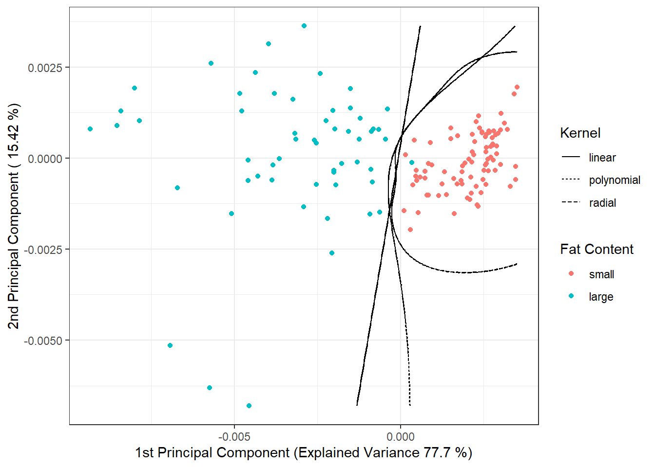 

Figure 5.33: Scores of the first two principal components, colored according to class membership. The decision boundary (line or curves in the plane of the first two principal components) between classes constructed using the SVM method is indicated in black.

Code

Res <- data.frame(model = c('SVM linear - PCA', 
                            'SVM poly - PCA', 
                            'SVM rbf - PCA'), 
                  Err.train = 1 - c(presnost.train.l, presnost.train.p, presnost.train.r),
                  Err.test = 1 - c(presnost.test.l, presnost.test.p, presnost.test.r))

RESULTS <- rbind(RESULTS, Res)

6.4.7.4 Basis Coefficients

Finally, we will use the representation of functions with a B-spline basis. For all three kernels, we will iterate over values of the hyperparameter \(C\) in the range \([10^{-4}, 10^{2}]\), while for the polynomial kernel, we will fix the hyperparameter \(p\) at the value of 3, as other integer values do not yield nearly as good results. Conversely, for the radial kernel, we will again use \(k_{cv}\)-fold cross-validation to choose the optimal value of the hyperparameter \(\gamma\), considering values in the range \([10^{-4}, 10^{0}]\). We will set coef0 = 1.

Code

set.seed(42)

# Values of gamma to consider
gamma.cv <- 10^seq(-4, 0, length = 5)
C.cv <- 10^seq(-4, 2, length = 7)
p.cv <- 3
coef0 <- 1

# List with three components ... arrays for each kernel -> linear, poly, radial
# Empty matrix to store results
# Columns will contain accuracy values for given parameters
# Rows will correspond to gamma values and layers will correspond to folds
CV.results <- list(
  SVM.l = array(NA, dim = c(length(C.cv), k_cv)),
  SVM.p = array(NA, dim = c(length(C.cv), length(p.cv), k_cv)),
  SVM.r = array(NA, dim = c(length(C.cv), length(gamma.cv), k_cv))
)

# First, iterate over values of C
for (C in C.cv) {
  # Iterate over each fold
  for (index_cv in 1:k_cv) {
    # Define test and training sets for CV
    fold <- folds[[index_cv]]
    cv_sample <- 1:dim(grid.data)[1] %in% fold
    
    data.Bbasis.train.cv <- as.data.frame(data.Bbasis.train[cv_sample, ])
    data.Bbasis.test.cv <- as.data.frame(data.Bbasis.train[!cv_sample, ])
    
    ## LINEAR KERNEL
    # Build the model
    clf.SVM.l <- svm(Y ~ ., data = data.Bbasis.train.cv,
                     type = 'C-classification',
                     scale = TRUE,
                     cost = C,
                     kernel = 'linear')
    
    # Accuracy on validation data
    predictions.test.l <- predict(clf.SVM.l, newdata = data.Bbasis.test.cv)
    presnost.test.l <- table(data.Bbasis.test.cv$Y, predictions.test.l) |>
      prop.table() |> diag() |> sum()
    
    # Store accuracy for the given C and fold
    CV.results$SVM.l[(1:length(C.cv))[C.cv == C], 
                     index_cv] <- presnost.test.l
    
    ## POLYNOMIAL KERNEL
    for (p in p.cv) {
      # Build the model
      clf.SVM.p <- svm(Y ~ ., data = data.Bbasis.train.cv,
                       type = 'C-classification',
                       scale = TRUE,
                       cost = C,
                       coef0 = coef0,
                       degree = p,
                       kernel = 'polynomial')
      
      # Accuracy on validation data
      predictions.test.p <- predict(clf.SVM.p, 
                                    newdata = data.Bbasis.test.cv)
      presnost.test.p <- table(data.Bbasis.test.cv$Y, predictions.test.p) |>
        prop.table() |> diag() |> sum()
      
      # Store accuracy for the given C, p, and fold
      CV.results$SVM.p[(1:length(C.cv))[C.cv == C], 
                       (1:length(p.cv))[p.cv == p],
                       index_cv] <- presnost.test.p
    }
        
    ## RADIAL KERNEL
    for (gamma in gamma.cv) {
      # Build the model
      clf.SVM.r <- svm(Y ~ ., data = data.Bbasis.train.cv,
                       type = 'C-classification',
                       scale = TRUE,
                       cost = C,
                       gamma = gamma,
                       kernel = 'radial')
      
      # Accuracy on validation data
      predictions.test.r <- predict(clf.SVM.r, 
                                    newdata = data.Bbasis.test.cv)
      presnost.test.r <- table(data.Bbasis.test.cv$Y, predictions.test.r) |>
        prop.table() |> diag() |> sum()
      
      # Store accuracy for the given C, gamma, and fold
      CV.results$SVM.r[(1:length(C.cv))[C.cv == C], 
                       (1:length(gamma.cv))[gamma.cv == gamma],
                       index_cv] <- presnost.test.r
    }
  }
}

Now, let’s average the results from \(k_{cv}\)-fold cross-validation so that we have one estimate of the validation error for each hyperparameter value (or combination of values). At the same time, we will determine the optimal values for each hyperparameter.

Code

# Calculate average accuracies for individual C across folds
## Linear kernel
CV.results$SVM.l <- apply(CV.results$SVM.l, 1, mean)
## Polynomial kernel
CV.results$SVM.p <- apply(CV.results$SVM.p, c(1, 2), mean)
## Radial kernel
CV.results$SVM.r <- apply(CV.results$SVM.r, c(1, 2), mean)

C.opt <- c(which.max(CV.results$SVM.l), 
           which.max(CV.results$SVM.p) %% length(C.cv), 
           which.max(CV.results$SVM.r) %% length(C.cv))
C.opt[C.opt == 0] <- length(C.cv)
C.opt <- C.cv[C.opt]

gamma.opt <- which.max(t(CV.results$SVM.r)) %% length(gamma.cv)
gamma.opt[gamma.opt == 0] <- length(gamma.cv)
gamma.opt <- gamma.cv[gamma.opt]

p.opt <- which.max(t(CV.results$SVM.p)) %% length(p.cv)
p.opt[p.opt == 0] <- length(p.cv)
p.opt <- p.cv[p.opt]

presnost.opt.cv <- c(max(CV.results$SVM.l), 
                     max(CV.results$SVM.p),
                     max(CV.results$SVM.r))

Let’s see how the optimal values turned out. For the linear kernel, the optimal value of \(C\) is 0.01, for the polynomial kernel \(C\) is 0.1, and for the radial kernel we have two optimal values: the optimal value for \(C\) is 100 and for \(\gamma\) it is 0.01. The validation errors are 0.0066667 for linear, 0.0133333 for polynomial, and 0.0066667 for radial kernels.

Finally, we can build the final classifiers on the entire training data using the hyperparameter values determined by \(k_{cv}\)-fold cross-validation. We will also determine the errors on the test and training datasets.

Code

# Build the models
clf.SVM.l.Bbasis <- svm(Y ~ ., data = data.Bbasis.train,
                        type = 'C-classification',
                        scale = TRUE,
                        cost = C.opt[1],
                        kernel = 'linear')

clf.SVM.p.Bbasis <- svm(Y ~ ., data = data.Bbasis.train,
                        type = 'C-classification',
                        scale = TRUE,
                        cost = C.opt[2],
                        degree = p.opt,
                        coef0 = coef0,
                        kernel = 'polynomial')

clf.SVM.r.Bbasis <- svm(Y ~ ., data = data.Bbasis.train,
                        type = 'C-classification',
                        scale = TRUE,
                        cost = C.opt[3],
                        gamma = gamma.opt,
                        kernel = 'radial')

# Accuracy on training data
predictions.train.l <- predict(clf.SVM.l.Bbasis, newdata = data.Bbasis.train)
presnost.train.l <- table(Y.train, predictions.train.l) |>
  prop.table() |> diag() |> sum()

predictions.train.p <- predict(clf.SVM.p.Bbasis, newdata = data.Bbasis.train)
presnost.train.p <- table(Y.train, predictions.train.p) |>
  prop.table() |> diag() |> sum()

predictions.train.r <- predict(clf.SVM.r.Bbasis, newdata = data.Bbasis.train)
presnost.train.r <- table(Y.train, predictions.train.r) |>
  prop.table() |> diag() |> sum()
  
# Accuracy on test data
predictions.test.l <- predict(clf.SVM.l.Bbasis, newdata = data.Bbasis.test)
presnost.test.l <- table(Y.test, predictions.test.l) |>
  prop.table() |> diag() |> sum()

predictions.test.p <- predict(clf.SVM.p.Bbasis, newdata = data.Bbasis.test)
presnost.test.p <- table(Y.test, predictions.test.p) |>
  prop.table() |> diag() |> sum()

predictions.test.r <- predict(clf.SVM.r.Bbasis, newdata = data.Bbasis.test)
presnost.test.r <- table(Y.test, predictions.test.r) |>
  prop.table() |> diag() |> sum()

The error of the SVM method applied to the basis coefficients on the training data is 0.67 % for the linear kernel, 0.67 % for the polynomial kernel, and 0 % for the radial kernel. On the test data, the error of the method is 7.6923 % for the linear kernel, 7.6923 % for the polynomial kernel, and 6.1538 % for the radial kernel.

Code

Res <- data.frame(model = c('SVM linear - Bbasis', 
                            'SVM poly - Bbasis', 
                            'SVM rbf - Bbasis'), 
                  Err.train = 1 - c(presnost.train.l, presnost.train.p, presnost.train.r),
                  Err.test = 1 - c(presnost.test.l, presnost.test.p, presnost.test.r))

RESULTS <- rbind(RESULTS, Res)

6.4.7.5 Projection onto B-spline Basis

Another option for applying the classical SVM method to functional data is to project the original data onto a \(d\)-dimensional subspace of our Hilbert space \(\mathcal H\), denoted as \(V_d\). Assume that this subspace \(V_d\) has an orthonormal basis \(\{\Psi_j\}_{j = 1, \dots, d}\). We define the transformation \(P_{V_d}\) as the orthogonal projection onto the subspace \(V_d\), which can be expressed as

\[ P_{V_d} (x) = \sum_{j = 1}^d \langle x, \Psi_j \rangle \Psi_j. \]

Now, we can use the coefficients from the orthogonal projection for classification, applying standard SVM to the vectors \(\left( \langle x, \Psi_1 \rangle, \dots, \langle x, \Psi_d \rangle\right)^\top\). By utilizing this transformation, we have defined a new, so-called adapted kernel, which consists of the orthogonal projection \(P_{V_d}\) and the kernel function of the standard support vector method. Thus, we have (adapted) kernel \(Q(x_i, x_j) = K(P_{V_d}(x_i), P_{V_d}(x_j))\). This is a method of dimension reduction, which we can refer to as filtering.

For the projection itself, we will use the project.basis() function from the fda library in R. Its input will be a matrix of original discrete (unsmoothed) data, the values in which we measure the values in the original data matrix, and the basis object onto which we want to project the data. We will choose projection onto a B-spline basis because the use of Fourier basis is not suitable for our non-periodic data.

The dimension \(d\) is chosen either from some prior expert knowledge or using cross-validation. In our case, we will determine the optimal dimension of the subspace \(V_d\) using \(k\)-fold cross-validation (choosing \(k \ll n\) due to the computational intensity of the method; often, \(k = 5\) or \(k = 10\) is chosen). We require B-splines of order 4; for the number of basis functions, the relationship is given by

\[ n_{basis} = n_{breaks} + n_{order} - 2, \]

where \(n_{breaks}\) is the number of knots and \(n_{order} = 4\). In R, however, the value of \(n_{basis}\) must be at least \(n_{order} = 4\), and for large values of \(n_{basis}\), overfitting of the model occurs, so we will choose a maximum of \(n_{basis}\) to be a smaller number, say 20.

Code

k_cv <- 10 # k-fold CV

# Values for B-spline basis
rangeval <- range(t)
norder <- 4
n_basis_min <- norder
n_basis_max <- 20

dimensions <- n_basis_min:n_basis_max # all dimensions we want to try

# Divide training data into k parts
folds <- createMultiFolds(1:sum(split), k = k_cv, time = 1)

# List with three components... matrices for individual kernels -> linear, poly, radial
# Empty matrix to insert individual results
# Columns will contain accuracy values for each part of the training set
# Rows will contain values for each dimension value
CV.results <- list(SVM.l = matrix(NA, nrow = length(dimensions), ncol = k_cv),
                   SVM.p = matrix(NA, nrow = length(dimensions), ncol = k_cv),
                   SVM.r = matrix(NA, nrow = length(dimensions), ncol = k_cv))

for (d in dimensions) {
  # Basis object
  bbasis <- create.bspline.basis(rangeval = rangeval, 
                                 nbasis = d)
  
  # Project discrete data onto B-spline basis of dimension d
  Projection <- project.basis(y = XX, # matrix of discrete data
                              argvals = t, # vector of arguments
                              basisobj = bbasis) # basis object
  
  # Split into training and testing data within CV
  XX.train <- subset(t(Projection), split == TRUE)
  
  for (index_cv in 1:k_cv) {
    # Define testing and training parts for CV
    fold <- folds[[index_cv]]
    cv_sample <- 1:dim(XX.train)[1] %in% fold
    
    data.projection.train.cv <- as.data.frame(XX.train[cv_sample, ])
    data.projection.train.cv$Y <- factor(Y.train[cv_sample])
    
    data.projection.test.cv <- as.data.frame(XX.train[!cv_sample, ])
    Y.test.cv <- Y.train[!cv_sample]
    data.projection.test.cv$Y <- factor(Y.test.cv)
  
    # Model construction
    clf.SVM.l.projection <- svm(Y ~ ., data = data.projection.train.cv,
                            type = 'C-classification',
                            scale = TRUE,
                            kernel = 'linear')
    
    clf.SVM.p.projection <- svm(Y ~ ., data = data.projection.train.cv,
                            type = 'C-classification',
                            scale = TRUE,
                            coef0 = coef0,
                            kernel = 'polynomial')
    
    clf.SVM.r.projection <- svm(Y ~ ., data = data.projection.train.cv,
                            type = 'C-classification',
                            scale = TRUE,
                            kernel = 'radial')
      
    # Accuracy on validation data
    ## linear kernel
    predictions.test.l <- predict(clf.SVM.l.projection,
                                  newdata = data.projection.test.cv)
    presnost.test.l <- table(Y.test.cv, predictions.test.l) |>
      prop.table() |> diag() |> sum()
    ## polynomial kernel
    predictions.test.p <- predict(clf.SVM.p.projection, 
                                  newdata = data.projection.test.cv)
    presnost.test.p <- table(Y.test.cv, predictions.test.p) |>
      prop.table() |> diag() |> sum()
    ## radial kernel
    predictions.test.r <- predict(clf.SVM.r.projection,
                                  newdata = data.projection.test.cv)
    presnost.test.r <- table(Y.test.cv, predictions.test.r) |>
      prop.table() |> diag() |> sum()
    
    # Insert accuracies into positions for given d and fold
    CV.results$SVM.l[d - min(dimensions) + 1, index_cv] <- presnost.test.l
    CV.results$SVM.p[d - min(dimensions) + 1, index_cv] <- presnost.test.p
    CV.results$SVM.r[d - min(dimensions) + 1, index_cv] <- presnost.test.r
  }
}
  
# Calculate average accuracies for each d across folds
for (n_method in 1:length(CV.results)) {
  CV.results[[n_method]] <- apply(CV.results[[n_method]], 1, mean)
}

d.opt <- c(which.max(CV.results$SVM.l) + n_basis_min - 1, 
           which.max(CV.results$SVM.p) + n_basis_min - 1, 
           which.max(CV.results$SVM.r) + n_basis_min - 1)
presnost.opt.cv <- c(max(CV.results$SVM.l), 
                     max(CV.results$SVM.p),
                     max(CV.results$SVM.r))
data.frame(d_opt = d.opt, ERR = 1 - presnost.opt.cv,
           row.names = c('linear', 'poly', 'radial'))

##        d_opt        ERR
## linear     9 0.01958333
## poly       7 0.03297619
## radial     6 0.14125000

We see that the optimal value of the parameter \(d\) is 9 for the linear kernel, with an error rate calculated using 10-fold CV of 0.0196, 7 for the polynomial kernel with an error rate of 0.033, and 6 for the radial kernel with an error rate of 0.1412.

To clarify, let’s plot the validation error rates as a function of the dimension \(d\).

Code

CV.results <- data.frame(d = dimensions |> rep(3), 
                         CV = c(CV.results$SVM.l, 
                                CV.results$SVM.p, 
                                CV.results$SVM.r),
                         Kernel = rep(c('linear', 'polynomial', 'radial'), 
                                      each = length(dimensions)) |> factor())
CV.results |> ggplot(aes(x = d, y = 1 - CV, colour = Kernel)) + 
  geom_line(linetype = 'dashed') + 
  geom_point(size = 1.5) + 
  geom_point(data = data.frame(d.opt,
                               presnost.opt.cv),
             aes(x = d.opt, y = 1 - presnost.opt.cv), colour = 'black', size = 2) +
  theme_bw() + 
  labs(x = bquote(paste(d)),
       y = 'Validation error rate',
       colour = 'Kernel') + 
  theme(legend.position = "bottom") + 
  scale_x_continuous(breaks = dimensions)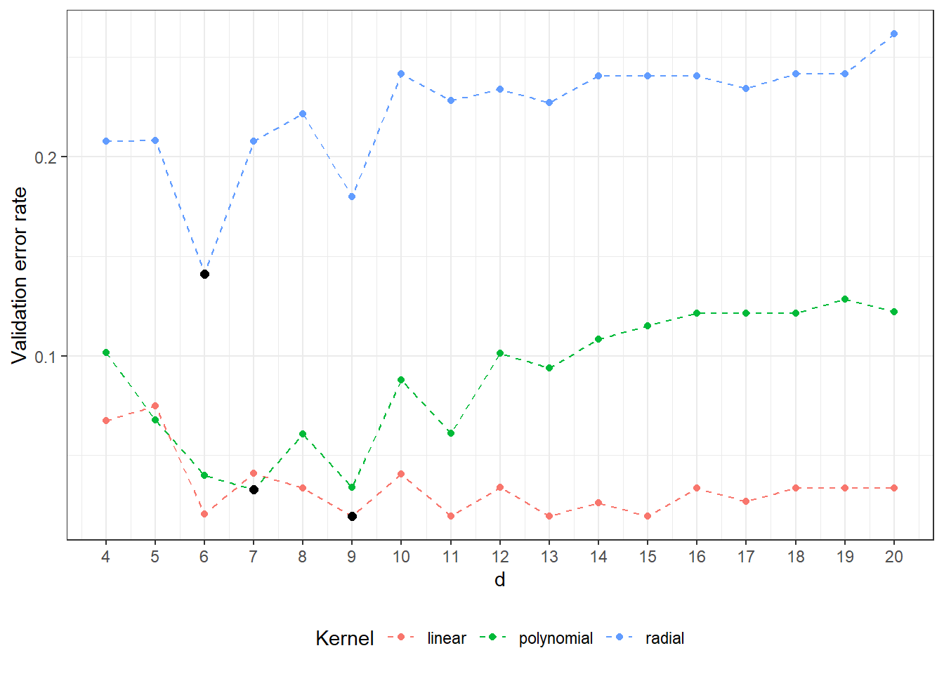

Figure 6.16: Dependency of validation error on the dimension of the subspace \(V_d\), separately for all three considered kernels in the SVM method. The black points indicate the optimal dimension values \(V_d\) for each kernel function.

Now we can train individual classifiers on all training data and examine their performance on the test data. For each kernel function, we choose the dimension of the subspace to project onto based on the results of cross-validation.

In the variable Projection, we have stored the matrix of orthogonal projection coefficients, given by

\[ \texttt{Projection} = \begin{pmatrix} \langle x_1, \Psi_1 \rangle & \langle x_2, \Psi_1 \rangle & \cdots & \langle x_n, \Psi_1 \rangle\\ \langle x_1, \Psi_2 \rangle & \langle x_2, \Psi_2 \rangle & \cdots & \langle x_n, \Psi_2 \rangle\\ \vdots & \vdots & \ddots & \vdots \\ \langle x_1, \Psi_d \rangle & \langle x_2, \Psi_d \rangle & \dots & \langle x_n, \Psi_d \rangle \end{pmatrix}_{d \times n}. \]

Code

# Prepare a data frame to store results
Res <- data.frame(model = c('SVM linear - projection', 
                             'SVM poly - projection', 
                             'SVM rbf - projection'), 
                  Err.train = NA,
                  Err.test = NA)

# Iterate through the kernels
for (kernel_number in 1:3) {
  kernel_type <- c('linear', 'polynomial', 'radial')[kernel_number]
  # Basis object
  bbasis <- create.bspline.basis(rangeval = rangeval, 
                                 nbasis = d.opt[kernel_number])
  
  # Project discrete data onto B-spline basis
  Projection <- project.basis(y = XX, # matrix of discrete data
                              argvals = t, # vector of arguments
                              basisobj = bbasis) # basis object
  
  # Split into training and test data
  XX.train <- subset(t(Projection), split == TRUE)
  XX.test <- subset(t(Projection), split == FALSE)
  
  data.projection.train <- as.data.frame(XX.train)
  data.projection.train$Y <- factor(Y.train)
  
  data.projection.test <- as.data.frame(XX.test)
  data.projection.test$Y <- factor(Y.test)
  
  # Build the model
  clf.SVM.projection <- svm(Y ~ ., data = data.projection.train,
                            type = 'C-classification',
                            scale = TRUE,
                            coef0 = coef0,
                            kernel = kernel_type)
  
  # Accuracy on training data
  predictions.train <- predict(clf.SVM.projection, newdata = data.projection.train)
  presnost.train <- table(Y.train, predictions.train) |>
    prop.table() |> diag() |> sum()
    
  # Accuracy on test data
  predictions.test <- predict(clf.SVM.projection, newdata = data.projection.test)
  presnost.test <- table(Y.test, predictions.test) |>
    prop.table() |> diag() |> sum()
  
  # Store the results
  Res[kernel_number, c(2, 3)] <- 1 - c(presnost.train, presnost.test)
}

The error rate of the SVM method applied to the basis coefficients on the training data is 2 % for the linear kernel, 2.67 % for the polynomial kernel, and 9.33 % for the Gaussian kernel. The error rate on the test data is 6.15 % for the linear kernel, 6.15 % for the polynomial kernel, and 10.77 % for the radial kernel.

Code

RESULTS <- rbind(RESULTS, Res)

6.4.7.6 RKHS + SVM

In this section, we will explore another way to use the support vector machine (SVM) method for classifying functional data. In this case, we will once again apply a known principle where we first express functional data as finite-dimensional objects, and then apply the classical SVM method to these objects.

From the last part of Theorem 1.3, we see how to compute curve representations in practice. We will work with discretized data after smoothing the curves. First, we define the kernel for the RKHS space. We will use the Gaussian kernel with parameter \(\gamma\). The value of this hyperparameter significantly influences the behavior and success of the method, so we must pay special attention to its choice (we choose it using cross-validation).

Code

# hyperparameter values same as in the previous section
eps <- 0.01
C <- 1 

6.4.7.6.0.1 Gaussian Kernel

Code

# remove the last column containing values of Y
data.RKHS <- grid.data[, -dim(grid.data)[2]] |> t()
# add test data as well
data.RKHS <- cbind(data.RKHS, grid.data.test[, -dim(grid.data.test)[2]] |> t())

# kernel and kernel matrix ... Gaussian with parameter gamma
Gauss.kernel <- function(x, y, gamma) {
  return(exp(-gamma * norm(c(x - y) |> t(), type = 'F')))
}

Kernel.RKHS <- function(x, gamma) {
  K <- matrix(NA, ncol = length(x), nrow = length(x))
  for(i in 1:nrow(K)) {
    for(j in 1:ncol(K)) {
      K[i, j] <- Gauss.kernel(x = x[i], y = x[j], gamma = gamma)
    }
  }
  return(K)
}

Now let’s compute the matrix \(K_S\) and its eigenvalues and corresponding eigenvectors.

Code

# compute matrix K
gamma <- 0.1 # fixed value of gamma, optimal value determined via CV
K <- Kernel.RKHS(t.seq, gamma = gamma)

# determine eigenvalues and eigenvectors
Eig <- eigen(K)
eig.vals <- Eig$values
eig.vectors <- Eig$vectors

To calculate the coefficients in the representation of the curves, i.e., the vectors \(\hat{\boldsymbol \lambda}_l^* = \left( \hat\lambda_{1l}^*, \dots, \hat\lambda_{\hat dl}^*\right)^\top, l = 1, 2, \dots, n\), we need the coefficients from the SVM. Unlike the classification problem, we now solve a regression problem, as we aim to express our observed curves in a basis chosen by the kernel \(K\). Therefore, we use the Support Vector Regression method, from which we subsequently obtain the coefficients \(\alpha_{il}\).

Code

# determine the alpha coefficients from SVM
alpha.RKHS <- matrix(0, nrow = dim(data.RKHS)[1],
                     ncol = dim(data.RKHS)[2]) # empty object

# model
for(i in 1:dim(data.RKHS)[2]) {
  df.svm <- data.frame(x = t.seq,
                       y = data.RKHS[, i])
  svm.RKHS <- svm(y ~ x, data = df.svm, 
                  kernel = 'radial',
                  type = 'eps-regression',
                  epsilon = eps,
                  cost = C,
                  gamma = gamma)
  # determine alpha
  alpha.RKHS[svm.RKHS$index, i] <- svm.RKHS$coefs # replace zeros with coefficients
}

Now we can compute the representations of the individual curves. First, we choose \(\hat d\) to be the entire dimension, i.e., \(\hat d = m ={}\) 101, and then we determine the optimal \(\hat d\) using cross-validation.

Code

# d
d.RKHS <- dim(alpha.RKHS)[1]

# determine the lambda vector
Lambda.RKHS <- matrix(NA, 
                      ncol = dim(data.RKHS)[2], 
                      nrow = d.RKHS) # create an empty object

# compute the representation
for(l in 1:dim(data.RKHS)[2]) {
  Lambda.RKHS[, l] <- (t(eig.vectors[, 1:d.RKHS]) %*% alpha.RKHS[, l]) * eig.vals[1:d.RKHS]
}

Now we have the matrix Lambda.RKHS storing the vectors \(\hat{\boldsymbol \lambda}_l^*, l = 1, 2, \dots, n\) in its columns for each curve. These vectors will be used as representations of the curves, and we will classify the data based on this discretization.

Code

# split into training and testing data
XX.train <- Lambda.RKHS[, 1:dim(grid.data)[1]]
XX.test <- Lambda.RKHS[, (dim(grid.data)[1] + 1):dim(Lambda.RKHS)[2]]

# prepare a data table to store results
Res <- data.frame(model = c('SVM linear - RKHS', 
                            'SVM poly - RKHS', 
                            'SVM rbf - RKHS'), 
                  Err.train = NA,
                  Err.test = NA)

# iterate over different kernels
for (kernel_number in 1:3) {
  kernel_type <- c('linear', 'polynomial', 'radial')[kernel_number]

  data.RKHS.train <- as.data.frame(t(XX.train))
  data.RKHS.train$Y <- factor(Y.train)
  
  data.RKHS.test <- as.data.frame(t(XX.test))
  data.RKHS.test$Y <- factor(Y.test)
  
  # construct the model
  clf.SVM.RKHS <- svm(Y ~ ., data = data.RKHS.train,
                      type = 'C-classification',
                      cost = C,
                      coef0 = coef0,
                      scale = TRUE,
                      kernel = kernel_type)
  
  # accuracy on training data
  predictions.train <- predict(clf.SVM.RKHS, newdata = data.RKHS.train)
  presnost.train <- table(Y.train, predictions.train) |>
    prop.table() |> diag() |> sum()
    
  # accuracy on test data
  predictions.test <- predict(clf.SVM.RKHS, newdata = data.RKHS.test)
  presnost.test <- table(Y.test, predictions.test) |>
    prop.table() |> diag() |> sum()
  
  # store results
  Res[kernel_number, c(2, 3)] <- 1 - c(presnost.train, presnost.test)
}

Table 6.9: Summary results of the SVM method combined with RKHS on simulated data. \(\widehat{Err}_{train}\) indicates the estimate of training error and \(\widehat{Err}_{test}\) indicates the testing error.

Model	\(\widehat{Err}_{train}\quad\quad\quad\quad\quad\)	\(\widehat{Err}_{test}\quad\quad\quad\quad\quad\)
SVM linear - RKHS	0	0
SVM poly - RKHS	0	0
SVM rbf - RKHS	0	0

We see that the model classifies the training data very well for all three kernels, while its performance on the test data is quite poor. It is evident that overfitting has occurred; therefore, we will use cross-validation to determine the optimal values for \(\gamma\) and \(d\).

Code

# Split training data into k parts
folds <- createMultiFolds(1:sum(split), k = k_cv, time = 1)
# Remove the last column, which contains the Y values
data.RKHS <- grid.data[, -dim(grid.data)[2]] |> t()

# Hyperparameter values to iterate over
dimensions <- 3:30 # reasonable range of values for d
gamma.cv <- 10^seq(-2, 2, length = 15)

# List with three components ... array for each kernel -> linear, poly, radial
# Empty matrix to store results
# Columns will contain accuracy values for given parameters
# Rows will contain values for given gamma, and layers correspond to folds
dim.names <- list(gamma = paste0('gamma:', round(gamma.cv, 3)),
                  d = paste0('d:', dimensions),
                  CV = paste0('cv:', 1:k_cv))

CV.results <- list(
  SVM.l = array(NA, dim = c(length(gamma.cv), length(dimensions), k_cv),
                dimnames = dim.names),
  SVM.p = array(NA, dim = c(length(gamma.cv), length(dimensions), k_cv),
                dimnames = dim.names),
  SVM.r = array(NA, dim = c(length(gamma.cv), length(dimensions), k_cv),
                dimnames = dim.names))

Code

# Cross-validation itself
for (gamma in gamma.cv) {
  K <- Kernel.RKHS(t.seq, gamma = gamma)
  Eig <- eigen(K)
  eig.vals <- Eig$values
  eig.vectors <- Eig$vectors
  alpha.RKHS <- matrix(0, nrow = dim(data.RKHS)[1], ncol = dim(data.RKHS)[2]) 
  
  # Model
  for(i in 1:dim(data.RKHS)[2]) {
    df.svm <- data.frame(x = t.seq,
                         y = data.RKHS[, i])
    svm.RKHS <- svm(y ~ x, data = df.svm, 
                    kernel = 'radial',
                    type = 'eps-regression',
                    epsilon = eps,
                    cost = C,
                    gamma = gamma)
    alpha.RKHS[svm.RKHS$index, i] <- svm.RKHS$coefs 
  }
  
  # Iterate over dimensions
  for(d.RKHS in dimensions) {
    Lambda.RKHS <- matrix(NA, 
                          ncol = dim(data.RKHS)[2], 
                          nrow = d.RKHS) 
    # Calculate representation
    for(l in 1:dim(data.RKHS)[2]) {
      Lambda.RKHS[, l] <- (t(eig.vectors[, 1:d.RKHS]) %*% 
                             alpha.RKHS[, l]) * eig.vals[1:d.RKHS]
    }
    # Iterate over folds
    for (index_cv in 1:k_cv) {
      # Define test and training portions for CV
      fold <- folds[[index_cv]]
      # Split into training and validation data
      XX.train <- Lambda.RKHS[, fold]
      XX.test <- Lambda.RKHS[, !(1:dim(Lambda.RKHS)[2] %in% fold)]
      # Prepare a data table to store results
      Res <- data.frame(model = c('SVM linear - RKHS', 
                                  'SVM poly - RKHS', 
                                  'SVM rbf - RKHS'), 
                        Err.test = NA)
      # Iterate over kernels
      for (kernel_number in 1:3) {
        kernel_type <- c('linear', 'polynomial', 'radial')[kernel_number]
      
        data.RKHS.train <- as.data.frame(t(XX.train))
        data.RKHS.train$Y <- factor(Y.train[fold])
        
        data.RKHS.test <- as.data.frame(t(XX.test))
        data.RKHS.test$Y <- factor(Y.train[!(1:dim(Lambda.RKHS)[2] %in% fold)])
        
        # Constructing the model
        clf.SVM.RKHS <- svm(Y ~ ., data = data.RKHS.train,
                            type = 'C-classification',
                            scale = TRUE,
                            cost = C,
                            coef0 = coef0,
                            kernel = kernel_type)
        
        # Accuracy on validation data
        predictions.test <- predict(clf.SVM.RKHS, newdata = data.RKHS.test)
        presnost.test <- table(data.RKHS.test$Y, predictions.test) |>
          prop.table() |> diag() |> sum()
        
        # Store results
        Res[kernel_number, 2] <- 1 - presnost.test
      }
      # Store accuracies in the positions for given d, gamma, and fold
      CV.results$SVM.l[paste0('gamma:', round(gamma, 3)), 
                       d.RKHS - min(dimensions) + 1, 
                       index_cv] <- Res[1, 2]
      CV.results$SVM.p[paste0('gamma:', round(gamma, 3)), 
                       d.RKHS - min(dimensions) + 1, 
                       index_cv] <- Res[2, 2]
      CV.results$SVM.r[paste0('gamma:', round(gamma, 3)), 
                       d.RKHS - min(dimensions) + 1, 
                       index_cv] <- Res[3, 2]
    }
  }
}

Code

# Calculate the average accuracy for each d across folds
for (n_method in 1:length(CV.results)) {
  CV.results[[n_method]] <- apply(CV.results[[n_method]], c(1, 2), mean)
}

gamma.opt <- c(which.min(CV.results$SVM.l) %% length(gamma.cv), 
               which.min(CV.results$SVM.p) %% length(gamma.cv), 
               which.min(CV.results$SVM.r) %% length(gamma.cv))
gamma.opt[gamma.opt == 0] <- length(gamma.cv)
gamma.opt <- gamma.cv[gamma.opt]

d.opt <- c(which.min(t(CV.results$SVM.l)) %% length(dimensions), 
           which.min(t(CV.results$SVM.p)) %% length(dimensions), 
           which.min(t(CV.results$SVM.r)) %% length(dimensions))
d.opt[d.opt == 0] <- length(dimensions)
d.opt <- dimensions[d.opt]

err.opt.cv <- c(min(CV.results$SVM.l), 
                 min(CV.results$SVM.p),
                 min(CV.results$SVM.r))
df.RKHS.res <- data.frame(d = d.opt, gamma = gamma.opt, CV = err.opt.cv,
                           Kernel = c('linear', 'polynomial', 'radial') |> factor(),
                           row.names = c('linear', 'poly', 'radial'))

Table 6.10: Summary results of cross-validation for the SVM method combined with RKHS on simulated data. \(\widehat{Err}_{train}\) denotes the estimate of training error and \(\widehat{Err}_{test}\) denotes test error.

	\(\quad\quad\quad\quad\quad d\)	\(\quad\quad\quad\quad\quad\gamma\)	\(\widehat{Err}_{cross\_validation}\)	Model
linear	12	1.0000	0	linear
poly	18	1.0000	0	polynomial
radial	17	1.9307	0	radial

We see that the best parameter values are \(d={}\) 12 and \(\gamma={}\) 1 for the linear kernel, with an error rate calculated using 10-fold CV of 0. The optimal values for \(d={}\) 18 and \(\gamma={}\) 1 correspond to the polynomial kernel, with an error rate of 0, and for \(d={}\) 17 and \(\gamma={}\) 1.9307 for the radial kernel, yielding an error rate of 0.

For interest, let’s plot the validation error as a function of dimension \(d\) and hyperparameter \(\gamma\).

Code

CV.results.plot <- data.frame(d = rep(dimensions |> rep(3), each = length(gamma.cv)), 
                              gamma = rep(gamma.cv, length(dimensions)) |> rep(3),
                              CV = c(c(CV.results$SVM.l), 
                                     c(CV.results$SVM.p), 
                                     c(CV.results$SVM.r)),
                              Kernel = rep(c('linear', 'polynomial', 'radial'), 
                                           each = length(dimensions) * 
                                             length(gamma.cv)) |> factor())
CV.results.plot |> 
  ggplot(aes(x = d, y = gamma, z = CV)) + 
  geom_contour_filled() +
  scale_y_continuous(trans='log10') +
  facet_wrap(~Kernel) +
  theme_bw() + 
  labs(x = expression(d),
       y = expression(gamma)) + 
  scale_fill_brewer(palette = "Spectral") + 
  geom_point(data = df.RKHS.res, aes(x = d, y = gamma),
             size = 5, pch = '+')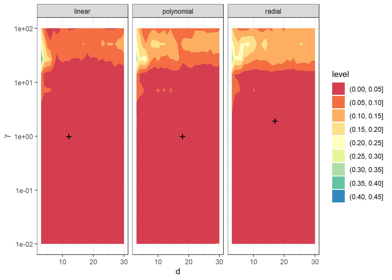

Figure 6.17: Dependency of validation error on the choice of hyperparameters \(d\) and \(\gamma\), separately for all three considered kernels in the SVM method.

Since we have already found the optimal hyperparameter values, we can construct the final models and assess their classification performance on the test data.

Code

# Remove the last column, which contains the values of Y
data.RKHS <- grid.data[, -dim(grid.data)[2]] |> t()
# Add the test data as well
data.RKHS <- cbind(data.RKHS, grid.data.test[, -dim(grid.data.test)[2]] |> t())

Code

# Prepare a data frame to store the results
Res <- data.frame(model = c('SVM linear - RKHS - radial', 
                             'SVM poly - RKHS - radial', 
                             'SVM rbf - RKHS - radial'), 
                  Err.train = NA,
                  Err.test = NA)

# Iterate through the individual kernels
for (kernel_number in 1:3) {
  # Calculate the K matrix
  gamma <- gamma.opt[kernel_number] # gamma value from CV
  K <- Kernel.RKHS(t.seq, gamma = gamma)
  
  # Determine eigenvalues and eigenvectors
  Eig <- eigen(K)
  eig.vals <- Eig$values
  eig.vectors <- Eig$vectors
  # Determine alpha coefficients from SVM
  alpha.RKHS <- matrix(0, nrow = dim(data.RKHS)[1],
                       ncol = dim(data.RKHS)[2]) # empty object
  
  # Model
  for(i in 1:dim(data.RKHS)[2]) {
    df.svm <- data.frame(x = t.seq,
                         y = data.RKHS[, i])
    svm.RKHS <- svm(y ~ x, data = df.svm, 
                    kernel = 'radial',
                    type = 'eps-regression',
                    epsilon = eps,
                    cost = C,
                    gamma = gamma)
    # Determine alpha
    alpha.RKHS[svm.RKHS$index, i] <- svm.RKHS$coefs # replace zeros with coefficients
  }
  # d
  d.RKHS <- d.opt[kernel_number]
  
  # Determine the lambda vector
  Lambda.RKHS <- matrix(NA, 
                        ncol = dim(data.RKHS)[2], 
                        nrow = d.RKHS) # create empty object
  
  # Calculate the representation
  for(l in 1:dim(data.RKHS)[2]) {
    Lambda.RKHS[, l] <- (t(eig.vectors[, 1:d.RKHS]) %*% alpha.RKHS[, l]) * eig.vals[1:d.RKHS]
  }
  
  # Split into training and test data
  XX.train <- Lambda.RKHS[, 1:dim(grid.data)[1]]
  XX.test <- Lambda.RKHS[, (dim(grid.data)[1] + 1):dim(Lambda.RKHS)[2]]

  kernel_type <- c('linear', 'polynomial', 'radial')[kernel_number]

  data.RKHS.train <- as.data.frame(t(XX.train))
  data.RKHS.train$Y <- factor(Y.train)
  
  data.RKHS.test <- as.data.frame(t(XX.test))
  data.RKHS.test$Y <- factor(Y.test)
  
  # Build models
  clf.SVM.RKHS <- svm(Y ~ ., data = data.RKHS.train,
                      type = 'C-classification',
                      scale = TRUE,
                      cost = C,
                      coef0 = coef0,
                      kernel = kernel_type)
  
  # Accuracy on training data
  predictions.train <- predict(clf.SVM.RKHS, newdata = data.RKHS.train)
  accuracy.train <- table(Y.train, predictions.train) |>
    prop.table() |> diag() |> sum()
    
  # Accuracy on test data
  predictions.test <- predict(clf.SVM.RKHS, newdata = data.RKHS.test)
  accuracy.test <- table(Y.test, predictions.test) |>
    prop.table() |> diag() |> sum()
  
  # Store results
  Res[kernel_number, c(2, 3)] <- 1 - c(accuracy.train, accuracy.test)
}

Table 6.11: Summary of SVM method results combined with RKHS on simulated data. \(\widehat{Err}_{train}\) denotes the estimate of training error and \(\widehat{Err}_{test}\) denotes testing error.

Model	\(\widehat{Err}_{train}\quad\quad\quad\quad\quad\)	\(\widehat{Err}_{test}\quad\quad\quad\quad\quad\)
SVM linear - RKHS - radial	0	0.0308
SVM poly - RKHS - radial	0	0.0769
SVM rbf - RKHS - radial	0	0.0308

The accuracy of the SVM method combined with projection onto Reproducing Kernel Hilbert Space is thus equal to 0 % for the linear kernel, 0 % for the polynomial kernel, and 0 % for the Gaussian kernel on the training data. On the test data, the accuracy of the method is 3.08 % for the linear kernel, 7.69 % for the polynomial kernel, and 3.08 % for the radial kernel.

Code

RESULTS <- rbind(RESULTS, Res)

6.4.7.6.0.2 Polynomial Kernel

Code

# Remove the last column containing Y values
data.RKHS <- grid.data[, -dim(grid.data)[2]] |> t()
# Add the test data as well
data.RKHS <- cbind(data.RKHS, grid.data.test[, -dim(grid.data.test)[2]] |> t())

# Kernel and kernel matrix ... polynomial with parameter p
Poly.kernel <- function(x, y, p) {
  return((1 + x * y)^p)
}

Kernel.RKHS <- function(x, p) {
  K <- matrix(NA, ncol = length(x), nrow = length(x))
  for(i in 1:nrow(K)) {
    for(j in 1:ncol(K)) {
      K[i, j] <- Poly.kernel(x = x[i], y = x[j], p)
    }
  }
  return(K)
}

Code

# Split training data into k parts
folds <- createMultiFolds(1:sum(split), k = k_cv, time = 1)
# Remove the last column containing Y values
data.RKHS <- grid.data[, -dim(grid.data)[2]] |> t()

# Values of hyperparameters to be searched
dimensions <- 2:30 # reasonable range of values d
poly.cv <- 2:5

# List with three components ... array for individual kernels -> linear, poly, radial
# Empty matrix where we will store individual results
# In columns will be the accuracy values for the given
# In rows will be values for given p and layers corresponding to folds
dim.names <- list(p = paste0('p:', poly.cv),
                  d = paste0('d:', dimensions),
                  CV = paste0('cv:', 1:k_cv))

CV.results <- list(
  SVM.l = array(NA, dim = c(length(poly.cv), length(dimensions), k_cv),
                dimnames = dim.names),
  SVM.p = array(NA, dim = c(length(poly.cv), length(dimensions), k_cv),
                dimnames = dim.names),
  SVM.r = array(NA, dim = c(length(poly.cv), length(dimensions), k_cv),
                dimnames = dim.names))

Code

# Actual CV
for (p in poly.cv) {
  K <- Kernel.RKHS(t.seq, p = p)
  Eig <- eigen(K)
  eig.vals <- Eig$values
  eig.vectors <- Eig$vectors
  alpha.RKHS <- matrix(0, nrow = dim(data.RKHS)[1], ncol = dim(data.RKHS)[2]) 
  
  # Model
  for(i in 1:dim(data.RKHS)[2]) {
    df.svm <- data.frame(x = t.seq,
                         y = data.RKHS[, i])
    svm.RKHS <- svm(y ~ x, data = df.svm, 
                    kernel = 'polynomial',
                    type = 'eps-regression',
                    coef0 = 1,
                    cost = C,
                    epsilon = eps,
                    degree = p)
    alpha.RKHS[svm.RKHS$index, i] <- svm.RKHS$coefs 
  }
  
  # Loop through dimensions
  for(d.RKHS in dimensions) {
    Lambda.RKHS <- matrix(NA, 
                          ncol = dim(data.RKHS)[2], 
                          nrow = d.RKHS) 
    # Compute representation
    for(l in 1:dim(data.RKHS)[2]) {
      Lambda.RKHS[, l] <- (t(eig.vectors[, 1:d.RKHS]) %*% 
                             alpha.RKHS[, l]) * eig.vals[1:d.RKHS]
    }
    # Loop through folds
    for (index_cv in 1:k_cv) {
      # Define test and training parts for CV
      fold <- folds[[index_cv]]
      # Split into training and validation data
      XX.train <- Lambda.RKHS[, fold]
      XX.test <- Lambda.RKHS[, !(1:dim(Lambda.RKHS)[2] %in% fold)]
      # Prepare a data table to store results
      Res <- data.frame(model = c('SVM linear - RKHS', 
                                  'SVM poly - RKHS', 
                                  'SVM rbf - RKHS'), 
                        Err.test = NA)
      # Loop through individual kernels
      for (kernel_number in 1:3) {
        kernel_type <- c('linear', 'polynomial', 'radial')[kernel_number]
      
        data.RKHS.train <- as.data.frame(t(XX.train))
        data.RKHS.train$Y <- factor(Y.train[fold])
        
        data.RKHS.test <- as.data.frame(t(XX.test))
        data.RKHS.test$Y <- factor(Y.train[!(1:dim(Lambda.RKHS)[2] %in% fold)])
        
        # Construct the model
        clf.SVM.RKHS <- svm(Y ~ ., data = data.RKHS.train,
                            type = 'C-classification',
                            scale = TRUE,
                            cost = C,                    
                            coef0 = 1,
                            gamma = 1,
                            kernel = kernel_type)
        
        # Accuracy on validation data
        predictions.test <- predict(clf.SVM.RKHS, newdata = data.RKHS.test)
        presnost.test <- table(data.RKHS.test$Y, predictions.test) |>
          prop.table() |> diag() |> sum()
        
        # Store results
        Res[kernel_number, 2] <- 1 - presnost.test
      }
      # Store accuracies at positions for given d, gamma, and fold
      CV.results$SVM.l[paste0('p:', p), 
                       d.RKHS - min(dimensions) + 1, 
                       index_cv] <- Res[1, 2]
      CV.results$SVM.p[paste0('p:', p), 
                       d.RKHS - min(dimensions) + 1, 
                       index_cv] <- Res[2, 2]
      CV.results$SVM.r[paste0('p:', p), 
                       d.RKHS - min(dimensions) + 1, 
                       index_cv] <- Res[3, 2]
    }
  }
}

Code

# Compute the average accuracies for each d across folds
for (n_method in 1:length(CV.results)) {
  CV.results[[n_method]] <- apply(CV.results[[n_method]], c(1, 2), mean)
}

poly.opt <- c(which.min(CV.results$SVM.l) %% length(poly.cv), 
               which.min(CV.results$SVM.p) %% length(poly.cv), 
               which.min(CV.results$SVM.r) %% length(poly.cv))
poly.opt[poly.opt == 0] <- length(poly.cv)
poly.opt <- poly.cv[poly.opt]

d.opt <- c(which.min(t(CV.results$SVM.l)) %% length(dimensions), 
           which.min(t(CV.results$SVM.p)) %% length(dimensions), 
           which.min(t(CV.results$SVM.r)) %% length(dimensions))
d.opt[d.opt == 0] <- length(dimensions)
d.opt <- dimensions[d.opt]

err.opt.cv <- c(min(CV.results$SVM.l), 
                 min(CV.results$SVM.p),
                 min(CV.results$SVM.r))
df.RKHS.res <- data.frame(d = d.opt, p = poly.opt, CV = err.opt.cv,
                           Kernel = c('linear', 'polynomial', 'radial') |> factor(),
                           row.names = c('linear', 'poly', 'radial'))

Table 6.12: Summary of cross-validation results for the SVM method combined with RKHS on simulated data. \(\widehat{Err}_{train}\) denotes the estimate of training error and \(\widehat{Err}_{test}\) the test error.

	\(\quad\quad\quad\quad\quad d\)	\(\quad\quad\quad\quad\quad p\)	\(\widehat{Err}_{cross\_validation}\)	Model
linear	30	3	0.0077	linear
poly	17	2	0.0077	polynomial
radial	3	4	0.0254	radial

We see that the optimal parameter values are \(d={}\) 30 and \(p={}\) 3 for the linear kernel with an error value computed using 10-fold CV 0.0077, \(d={}\) 17 and \(p={}\) 2 for the polynomial kernel with an error value computed using 10-fold CV 0.0077, and \(d={}\) 3 and \(p={}\) 4 for the radial kernel with an error value 0.0254.

Since we have found the optimal hyperparameter values, we can construct the final models and determine their classification success on the test data.

Code

# Remove the last column, which contains the Y values
data.RKHS <- grid.data[, -dim(grid.data)[2]] |> t()
# Add the test data
data.RKHS <- cbind(data.RKHS, grid.data.test[, -dim(grid.data.test)[2]] |> t())

Code

# Prepare a data frame to store results
Res <- data.frame(model = c('SVM linear - RKHS - poly', 
                             'SVM poly - RKHS - poly', 
                             'SVM rbf - RKHS - poly'), 
                  Err.train = NA,
                  Err.test = NA)

# Iterate through individual kernels
for (kernel_number in 1:3) {
  # Compute the K matrix
  p <- poly.opt[kernel_number] # gamma value using CV
  K <- Kernel.RKHS(t.seq, p = p)
  
  # Determine eigenvalues and eigenvectors
  Eig <- eigen(K)
  eig.vals <- Eig$values
  eig.vectors <- Eig$vectors
  # Determine alpha coefficients from SVM
  alpha.RKHS <- matrix(0, nrow = dim(data.RKHS)[1],
                       ncol = dim(data.RKHS)[2]) # empty object
  
  # Model
  for(i in 1:dim(data.RKHS)[2]) {
    df.svm <- data.frame(x = t.seq,
                         y = data.RKHS[, i])
    svm.RKHS <- svm(y ~ x, data = df.svm, 
                    kernel = 'polynomial',
                    type = 'eps-regression',
                    epsilon = eps,
                    coef0 = 1,
                    cost = C,
                    gamma = 1,
                    degree = p)
    # Determine alpha
    alpha.RKHS[svm.RKHS$index, i] <- svm.RKHS$coefs # replace zeros with coefficients
  }
  # d
  d.RKHS <- d.opt[kernel_number]
  
  # Determine the lambda vector
  Lambda.RKHS <- matrix(NA, 
                        ncol = dim(data.RKHS)[2], 
                        nrow = d.RKHS) # create an empty object
  
  # Compute the representation
  for(l in 1:dim(data.RKHS)[2]) {
    Lambda.RKHS[, l] <- (t(eig.vectors[, 1:d.RKHS]) %*% alpha.RKHS[, l]) * eig.vals[1:d.RKHS]
  }
  
  # Split into training and test data
  XX.train <- Lambda.RKHS[, 1:dim(grid.data)[1]]
  XX.test <- Lambda.RKHS[, (dim(grid.data)[1] + 1):dim(Lambda.RKHS)[2]]

  kernel_type <- c('linear', 'polynomial', 'radial')[kernel_number]

  data.RKHS.train <- as.data.frame(t(XX.train))
  data.RKHS.train$Y <- factor(Y.train)
  
  data.RKHS.test <- as.data.frame(t(XX.test))
  data.RKHS.test$Y <- factor(Y.test)
  
  # Construct models
  clf.SVM.RKHS <- svm(Y ~ ., data = data.RKHS.train,
                      type = 'C-classification',
                      scale = TRUE,
                      coef0 = 1,
                      cost = C,
                      gamma = 1,
                      kernel = kernel_type)
  
  # Accuracy on training data
  predictions.train <- predict(clf.SVM.RKHS, newdata = data.RKHS.train)
  accuracy.train <- table(Y.train, predictions.train) |>
    prop.table() |> diag() |> sum()
    
  # Accuracy on test data
  predictions.test <- predict(clf.SVM.RKHS, newdata = data.RKHS.test)
  accuracy.test <- table(Y.test, predictions.test) |>
    prop.table() |> diag() |> sum()
  
  # Save results
  Res[kernel_number, c(2, 3)] <- 1 - c(accuracy.train, accuracy.test)
}

Table 6.13: Summary of the SVM method combined with RKHS on simulated data. \(\widehat{Err}_{train}\) denotes the estimate of training error and \(\widehat{Err}_{test}\) the test error.

Model	\(\widehat{Err}_{train}\quad\quad\quad\quad\quad\)	\(\widehat{Err}_{test}\quad\quad\quad\quad\quad\)
SVM linear - RKHS - poly	0.00	0.0308
SVM poly - RKHS - poly	0.00	0.0154
SVM rbf - RKHS - poly	0.02	0.0308

The error rate of the SVM method combined with projection onto the Reproducing Kernel Hilbert Space is thus 0 % for the linear kernel, 0 % for the polynomial kernel, and 2 % for the Gaussian kernel. On the test data, the error rate of the method is 3.08 % for the linear kernel, 1.54 % for the polynomial kernel, and 3.08 % for the radial kernel.

Code

RESULTS <- rbind(RESULTS, Res)

6.4.7.6.0.3 Linear Kernel

Code

# remove the last column, which contains the Y values
data.RKHS <- grid.data[, -dim(grid.data)[2]] |> t()
# also add test data
data.RKHS <- cbind(data.RKHS, grid.data.test[, -dim(grid.data.test)[2]] |> t())

# kernel and kernel matrix ... polynomial with parameter p
Linear.kernel <- function(x, y) {
  return(x * y)
}

Kernel.RKHS <- function(x) {
  K <- matrix(NA, ncol = length(x), nrow = length(x))
  for(i in 1:nrow(K)) {
    for(j in 1:ncol(K)) {
      K[i, j] <- Linear.kernel(x = x[i], y = x[j])
    }
  }
  return(K)
}

Code

# split training data into k parts
folds <- createMultiFolds(1:sum(split), k = k_cv, time = 1)
# remove the last column, which contains the Y values
data.RKHS <- grid.data[, -dim(grid.data)[2]] |> t()

# hyperparameter values that we will iterate over
dimensions <- 2:40 # reasonable range of values for d

# list with three components ... array for individual kernels -> linear, poly, radial
# empty matrix into which we will insert the individual results
# in columns will be accuracy values for given d
# in rows will be values for layers corresponding to folds
dim.names <- list(d = paste0('d:', dimensions),
                  CV = paste0('cv:', 1:k_cv))

CV.results <- list(
  SVM.l = array(NA, dim = c(length(dimensions), k_cv),
                dimnames = dim.names),
  SVM.p = array(NA, dim = c(length(dimensions), k_cv),
                dimnames = dim.names),
  SVM.r = array(NA, dim = c(length(dimensions), k_cv),
                dimnames = dim.names))

Code

# the actual CV
K <- Kernel.RKHS(t.seq)
Eig <- eigen(K)
eig.vals <- Eig$values
eig.vectors <- Eig$vectors
alpha.RKHS <- matrix(0, nrow = dim(data.RKHS)[1], ncol = dim(data.RKHS)[2]) 

# model
for(i in 1:dim(data.RKHS)[2]) {
  df.svm <- data.frame(x = t.seq,
                       y = data.RKHS[, i])
  svm.RKHS <- svm(y ~ x, data = df.svm, 
                  kernel = 'linear',
                  type = 'eps-regression',
                  epsilon = eps,                   
                  coef0 = 1,
                  gamma = 1,
                  cost = C)
  alpha.RKHS[svm.RKHS$index, i] <- svm.RKHS$coefs 
}

# iterate through dimensions
for(d.RKHS in dimensions) {
  Lambda.RKHS <- matrix(NA, 
                        ncol = dim(data.RKHS)[2], 
                        nrow = d.RKHS) 
  # compute representation
  for(l in 1:dim(data.RKHS)[2]) {
    Lambda.RKHS[, l] <- (t(eig.vectors[, 1:d.RKHS]) %*% 
                           alpha.RKHS[, l]) * eig.vals[1:d.RKHS]
  }
  # iterate through folds
  for (index_cv in 1:k_cv) {
    # define test and training parts for CV
    fold <- folds[[index_cv]]
    # split into training and validation data
    XX.train <- Lambda.RKHS[, fold]
    XX.test <- Lambda.RKHS[, !(1:dim(Lambda.RKHS)[2] %in% fold)]
    # prepare a data table to store results
    Res <- data.frame(model = c('SVM linear - RKHS', 
                                'SVM poly - RKHS', 
                                'SVM rbf - RKHS'), 
                      Err.test = NA)
    # iterate through individual kernels
    for (kernel_number in 1:3) {
      kernel_type <- c('linear', 'polynomial', 'radial')[kernel_number]
    
      data.RKHS.train <- as.data.frame(t(XX.train))
      data.RKHS.train$Y <- factor(Y.train[fold])
      
      data.RKHS.test <- as.data.frame(t(XX.test))
      data.RKHS.test$Y <- factor(Y.train[!(1:dim(Lambda.RKHS)[2] %in% fold)])
      
      # model construction
      clf.SVM.RKHS <- svm(Y ~ ., data = data.RKHS.train,
                          type = 'C-classification',
                          scale = TRUE,
                          kernel = kernel_type,
                          epsilon = eps,                   
                          coef0 = 1,
                          gamma = 1,
                          cost = C)
      
      # accuracy on validation data
      predictions.test <- predict(clf.SVM.RKHS, newdata = data.RKHS.test)
      presnost.test <- table(data.RKHS.test$Y, predictions.test) |>
        prop.table() |> diag() |> sum()
      
      # store results
      Res[kernel_number, 2] <- 1 - presnost.test
    }
    # insert accuracies into positions for given d, gamma, and fold
    CV.results$SVM.l[d.RKHS - min(dimensions) + 1, 
                     index_cv] <- Res[1, 2]
    CV.results$SVM.p[d.RKHS - min(dimensions) + 1, 
                     index_cv] <- Res[2, 2]
    CV.results$SVM.r[d.RKHS - min(dimensions) + 1, 
                     index_cv] <- Res[3, 2]
  }
}

Code

# calculate the average accuracies for individual d across folds
for (n_method in 1:length(CV.results)) {
  CV.results[[n_method]] <- apply(CV.results[[n_method]], 1, mean)
}

d.opt <- c(which.min(t(CV.results$SVM.l)) %% length(dimensions), 
           which.min(t(CV.results$SVM.p)) %% length(dimensions), 
           which.min(t(CV.results$SVM.r)) %% length(dimensions))
d.opt[d.opt == 0] <- length(dimensions)
d.opt <- dimensions[d.opt]

err.opt.cv <- c(min(CV.results$SVM.l), 
                     min(CV.results$SVM.p),
                     min(CV.results$SVM.r))
df.RKHS.res <- data.frame(d = d.opt, CV = err.opt.cv,
           Kernel = c('linear', 'polynomial', 'radial') |> factor(),
           row.names = c('linear', 'poly', 'radial'))

Table 6.14: Summary of cross-validation results for the SVM method combined with RKHS on simulated data. \(\widehat{Err}_{train}\) denotes the estimate of training error and \(\widehat{Err}_{test}\) the test error.

	\(\quad\quad\quad\quad\quad d\)	\(\widehat{Err}_{cross\_validation}\)	Model
linear	31	0.0267	linear
poly	21	0.0267	polynomial
radial	6	0.0592	radial

We see that the optimal value of the parameter \(d={}\) 31 for the linear kernel yields a cross-validation error of 0.0267, \(d={}\) 21 for the polynomial kernel with a cross-validation error of 0.0267, and \(d={}\) 6 for the radial kernel with a cross-validation error of 0.0592.

Since we have already found the optimal values of the hyperparameters, we can construct the final models and determine their classification performance on the test data.

Code

# remove the last column, which contains the Y values
data.RKHS <- grid.data[, -dim(grid.data)[2]] |> t()
# add the test data
data.RKHS <- cbind(data.RKHS, grid.data.test[, -dim(grid.data.test)[2]] |> t())

Code

# prepare a data table to store the results
Res <- data.frame(model = c('SVM linear - RKHS - linear', 
                            'SVM poly - RKHS - linear', 
                            'SVM rbf - RKHS - linear'), 
                  Err.train = NA,
                  Err.test = NA)

# iterate over individual kernels
for (kernel_number in 1:3) {
  # calculate the K matrix
  K <- Kernel.RKHS(t.seq)
  
  # determine eigenvalues and eigenvectors
  Eig <- eigen(K)
  eig.vals <- Eig$values
  eig.vectors <- Eig$vectors
  # determine alpha coefficients from SVM
  alpha.RKHS <- matrix(0, nrow = dim(data.RKHS)[1],
                       ncol = dim(data.RKHS)[2]) # empty object
  
  # model
  for(i in 1:dim(data.RKHS)[2]) {
    df.svm <- data.frame(x = t.seq,
                         y = data.RKHS[, i])
    svm.RKHS <- svm(y ~ x, data = df.svm, 
                    kernel = 'linear',
                    type = 'eps-regression',
                    epsilon = eps,                   
                    coef0 = 1,
                    gamma = 1,
                    cost = C)
    # determine alpha
    alpha.RKHS[svm.RKHS$index, i] <- svm.RKHS$coefs # replace zeros with coefficients
  }
  # d
  d.RKHS <- d.opt[kernel_number]
  
  # determine the lambda vector
  Lambda.RKHS <- matrix(NA, 
                        ncol = dim(data.RKHS)[2], 
                        nrow = d.RKHS) # create an empty object
  
  # calculate the representation
  for(l in 1:dim(data.RKHS)[2]) {
    Lambda.RKHS[, l] <- (t(eig.vectors[, 1:d.RKHS]) %*% alpha.RKHS[, l]) * eig.vals[1:d.RKHS]
  }
  
  # split into training and test data
  XX.train <- Lambda.RKHS[, 1:dim(grid.data)[1]]
  XX.test <- Lambda.RKHS[, (dim(grid.data)[1] + 1):dim(Lambda.RKHS)[2]]

  kernel_type <- c('linear', 'polynomial', 'radial')[kernel_number]

  data.RKHS.train <- as.data.frame(t(XX.train))
  data.RKHS.train$Y <- factor(Y.train)
  
  data.RKHS.test <- as.data.frame(t(XX.test))
  data.RKHS.test$Y <- factor(Y.test)
  
  # build the models
  clf.SVM.RKHS <- svm(Y ~ ., data = data.RKHS.train,
                      type = 'C-classification',
                      scale = TRUE,
                      kernel = kernel_type,
                      epsilon = eps,                   
                      coef0 = 1,
                      gamma = 1,
                      cost = C)
  
  # accuracy on training data
  predictions.train <- predict(clf.SVM.RKHS, newdata = data.RKHS.train)
  accuracy.train <- table(Y.train, predictions.train) |>
    prop.table() |> diag() |> sum()
    
  # accuracy on test data
  predictions.test <- predict(clf.SVM.RKHS, newdata = data.RKHS.test)
  accuracy.test <- table(Y.test, predictions.test) |>
    prop.table() |> diag() |> sum()
  
  # save results
  Res[kernel_number, c(2, 3)] <- 1 - c(accuracy.train, accuracy.test)
}

Table 6.15: Summary of the SVM method combined with RKHS on simulated data. \(\widehat{Err}_{train}\) denotes the estimate of training error and \(\widehat{Err}_{test}\) the test error.

Model	\(\widehat{Err}_{train}\quad\quad\quad\quad\quad\)	\(\widehat{Err}_{test}\quad\quad\quad\quad\quad\)
SVM linear - RKHS - linear	0.00	0.0462
SVM poly - RKHS - linear	0.00	0.0308
SVM rbf - RKHS - linear	0.02	0.1231

The error rate of the SVM method combined with projection onto the Reproducing Kernel Hilbert Space is thus 0 % on the training data for the linear kernel, 0 % for the polynomial kernel, and 2 % for the Gaussian kernel. On the test data, the error rate is 4.62 % for the linear kernel, 3.08 % for the polynomial kernel, and 12.31 % for the radial kernel.

Code

RESULTS <- rbind(RESULTS, Res)

6.4.8 Results Table

From the table below, let us note two significant points. The first is that the methods classify the data significantly better than in the case of the original non-derivative data. In some methods, the improvement is even by tens of percent. The second significant point is that there is not such a pronounced difference between the results of the individual methods now.

Table 6.16: Summary of the results of the methods used on the simulated data. \(\widehat{Err}_{train}\) indicates the estimate of training error and \(\widehat{Err}_{test}\) of testing error.

Model	\(\widehat{Err}_{train}\quad\quad\quad\quad\quad\)	\(\widehat{Err}_{test}\quad\quad\quad\quad\quad\)
KNN	0.0133	0.0769
LDA	0.0400	0.0923
QDA	0.0067	0.0154
LR functional	0.0000	0.0769
LR score	0.0067	0.0462
Tree - discretization	0.0067	0.0154
Tree - score	0.0067	0.0615
Tree - Bbasis	0.0067	0.0154
RForest - diskr	0.0000	0.0462
RForest - score	0.0067	0.0462
RForest - Bbasis	0.0000	0.0308
SVM linear - func	0.0000	0.0308
SVM poly - func	0.0000	0.0000
SVM rbf - func	0.0000	0.0462
SVM linear - discr	0.0067	0.0154
SVM poly - discr	0.0067	0.0615
SVM rbf - discr	0.0000	0.0462
SVM linear - PCA	0.0067	0.0308
SVM poly - PCA	0.0067	0.0308
SVM rbf - PCA	0.0067	0.0154
SVM linear - Bbasis	0.0067	0.0769
SVM poly - Bbasis	0.0067	0.0769
SVM rbf - Bbasis	0.0000	0.0615
SVM linear - projection	0.0200	0.0615
SVM poly - projection	0.0267	0.0615
SVM rbf - projection	0.0933	0.1077
SVM linear - RKHS - radial	0.0000	0.0308
SVM poly - RKHS - radial	0.0000	0.0769
SVM rbf - RKHS - radial	0.0000	0.0308
SVM linear - RKHS - poly	0.0000	0.0308
SVM poly - RKHS - poly	0.0000	0.0154
SVM rbf - RKHS - poly	0.0200	0.0308
SVM linear - RKHS - linear	0.0000	0.0462
SVM poly - RKHS - linear	0.0000	0.0308
SVM rbf - RKHS - linear	0.0200	0.1231

6.5 Simulation Study

In the entire previous section, we dealt with a set of functions from two classification classes, which we then randomly split into testing and training parts. We then evaluated the individual classifiers obtained using the considered methods based on testing and training error rates.

Since the division of data into two parts can vary significantly with each repetition, the error rates of the individual classification algorithms will also differ significantly. Therefore, making any conclusions about the methods and comparing them to each other based on a single generated training dataset can be very misleading.

For this reason, this section will focus on repeating the entire previous procedure for different splits. We will store the results in a table and finally calculate the average characteristics of the models across the individual repetitions. To ensure our conclusions are sufficiently general, we will choose the number of repetitions \(n_{sim} = 100\).

Code

# Set different names for classification methods
methods_names <- c(
      '$K$ nearest neighbors',
      'Linear discriminant analysis',
      'Quadratic discriminant analysis',
      'Functional logistic regression',
      'Logistic regression with fPCA',
      'Decision tree -- discretization',
      'Decision tree -- fPCA',
      'Decision tree -- basis coefficients',
      'Random forest -- discretization',
      'Random forest -- fPCA',
      'Random forest -- basis coefficients',
      'SVM (linear) -- functional',
      'SVM (poly) -- functional',
      'SVM (radial) -- functional',
      'SVM (linear) -- discretization',
      'SVM (poly) -- discretization',
      'SVM (radial) -- discretization',
      'SVM (linear) -- fPCA',
      'SVM (poly) -- fPCA',
      'SVM (radial) -- fPCA',
      'SVM (linear) -- basis coefficients',
      'SVM (poly) -- basis coefficients',
      'SVM (radial) -- basis coefficients',
      'SVM (linear) -- projection',
      'SVM (poly) -- projection',
      'SVM (radial) -- projection',
      'RKHS (radial SVR) $+$ SVM (linear)',
      'RKHS (radial SVR) $+$ SVM (poly)',
      'RKHS (radial SVR) $+$ SVM (radial)',
      'RKHS (poly SVR) $+$ SVM (linear)',
      'RKHS (poly SVR) $+$ SVM (poly)',
      'RKHS (poly SVR) $+$ SVM (radial)',
      'RKHS (linear SVR) $+$ SVM (linear)',
      'RKHS (linear SVR) $+$ SVM (poly)',
      'RKHS (linear SVR) $+$ SVM (radial)'
)


# Colors for box plots 
box_col <- c('#4dd2ff', '#0099cc', '#00ace6', '#00bfff',
             '#1ac5ff', rep('#33ccff', 3), rep('#0086b3', 3), rep('#ff3814', 3),
             rep('#ff3814', 3), rep('#ff6347', 3), rep('#ff7961', 3),
             rep('#ff4d2e', 3), rep('#fa2600', 9))

# box_col <- c('#CA0A0A', '#fa2600', '#fa2600', '#D15804',
#              '#D15804', rep('#D3006D', 3), rep('#BE090F', 3), c("#12DEE8", "#4ECBF3", "#127DE8", "#4C3CD3", "#4E65F3", "#4E9EF3", "#081D58") |> rep(each = 3))

# Alpha for box plots
box_alpha <- c(0.9, 0.9, 0.8, 0.9, 0.8, 0.9, 0.8, 0.7, 0.9, 0.8, 0.7,
               0.9, 0.8, 0.7, 0.9, 0.8, 0.7, 0.9, 0.8, 0.7, 0.9, 0.8, 0.7, 0.9, 0.8, 0.7,
               seq(0.9, 0.6, length = 9)) #- 0.3

Code

# Set different names for classification methods
methods_names1 <- c(
      'KNN',
      'LDA',
      'QDA',
      'functional LR',
      'LR with fPCA',
      #'Decision Tree -- Discretization',
      #'Decision Tree -- fPCA',
      #'Decision Tree -- Basis Coefficients',
      'RF -- discretization',
      'RF -- fPCA',
      'RF -- basis coefficients',
      'SVM (linear) -- functional',
      'SVM (poly) -- functional',
      'SVM (radial) -- functional',
      'SVM (linear) -- discretization',
      'SVM (poly) -- discretization',
      'SVM (radial) -- discretization',
      'SVM (linear) -- fPCA',
      'SVM (poly) -- fPCA',
      'SVM (radial) -- fPCA',
      'SVM (linear) -- basis coefficients',
      'SVM (poly) -- basis coefficients',
      'SVM (radial) -- basis coefficients',
      'SVM (linear) -- projection',
      'SVM (poly) -- projection',
      'SVM (radial) -- projection',
      'RKHS (radial SVR) $+$ SVM (linear)',
      'RKHS (radial SVR) $+$ SVM (poly)',
      'RKHS (radial SVR) $+$ SVM (radial)',
      'RKHS (poly SVR) $+$ SVM (linear)',
      'RKHS (poly SVR) $+$ SVM (poly)',
      'RKHS (poly SVR) $+$ SVM (radial)'#,
      #'RKHS (Linear SVR) $+$ SVM (linear)',
      #'RKHS (Linear SVR) $+$ SVM (poly)',
      #'RKHS (Linear SVR) $+$ SVM (radial)'
)


# Colors for box plots 
box_col1 <- c('#4dd2ff', '#00ace6', '#00ace6', '#00bfff',  '#00bfff',
             rep('#0086b3', 3),
             rep('#ff3814', 3), rep('#ff3814', 3), rep('#ff3814', 3), rep('#ff6347', 3), rep('#ff7961', 3),
             rep('#ff4d2e', 3), rep('#fa2600', 3))

# alpha for box plots
box_alpha1 <- c(0.9, 0.9, 0.8, 0.9, 0.8, 0.9, 0.8, 0.7,
               rep(c(0.9, 0.8, 0.7), 7)) #- 0.3

6.5.1 Simulation for original Data

First, let us look at the simulation of the original, that is, non-derivative data.

Code

# setting the pseudorandom number generator
set.seed(42)

# number of simulations
n.sim <- 100

## list to store error values
# methods will be in the columns
# individual repetitions will be in the rows
# the list has two items ... train and test
methods <- c('KNN', 'LDA', 'QDA', 'LR_functional', 'LR_score', 'Tree_discr',
             'Tree_score', 'Tree_Bbasis', 'RF_discr', 'RF_score', 'RF_Bbasis',
             'SVM linear - func', 'SVM poly - func', 'SVM rbf - func',
             'SVM linear - discr', 'SVM poly - discr', 'SVM rbf - discr', 
             'SVM linear - PCA', 'SVM poly - PCA', 'SVM rbf - PCA', 
             'SVM linear - Bbasis', 'SVM poly - Bbasis', 'SVM rbf - Bbasis',
             'SVM linear - projection', 'SVM poly - projection', 
             'SVM rbf - projection', 'SVM linear - RKHS - radial', 
             'SVM poly - RKHS - radial', 'SVM rbf - RKHS - radial', 
             'SVM linear - RKHS - poly', 'SVM poly - RKHS - poly', 
             'SVM rbf - RKHS - poly', 'SVM linear - RKHS - linear', 
             'SVM poly - RKHS - linear', 'SVM rbf - RKHS - linear')

SIMULACE <- list(train = as.data.frame(matrix(NA, ncol = length(methods), 
                                             nrow = n.sim,
                                             dimnames = list(1:n.sim, methods))), 
                 test = as.data.frame(matrix(NA, ncol = length(methods), 
                                             nrow = n.sim,
                                             dimnames = list(1:n.sim, methods))))

# object to store optimal values of hyperparameters determined using CV
CV_RESULTS <- data.frame(KNN_K = rep(NA, n.sim), 
                         nharm = NA, 
                         LR_func_n_basis = NA,
                         SVM_d_Linear = NA,
                         SVM_d_Poly = NA,
                         SVM_d_Radial = NA, 
                         SVM_RKHS_radial_gamma1 = NA,
                         SVM_RKHS_radial_gamma2 = NA,
                         SVM_RKHS_radial_gamma3 = NA,
                         SVM_RKHS_radial_d1 = NA,
                         SVM_RKHS_radial_d2 = NA,
                         SVM_RKHS_radial_d3 = NA,
                         SVM_RKHS_poly_p1 = NA,
                         SVM_RKHS_poly_p2 = NA,
                         SVM_RKHS_poly_p3 = NA,
                         SVM_RKHS_poly_d1 = NA,
                         SVM_RKHS_poly_d2 = NA,
                         SVM_RKHS_poly_d3 = NA,
                         SVM_RKHS_linear_d1 = NA,
                         SVM_RKHS_linear_d2 = NA,
                         SVM_RKHS_linear_d3 = NA)

Now we will repeat the entire previous part 100 times and store the error values in the list SIMULACE. We will also save the optimal hyperparameter values in the data table CV_RESULTS—for the \(K\) nearest neighbors method and for SVM the dimension \(d\) in the case of projection onto the B-spline basis. We will also store all hyperparameter values for the SVM + RKHS method.

Code

# nastaveni generatoru pseudonahodnych cisel
set.seed(42)

## SIMULACE

for(sim in 1:n.sim) {
  # rozdeleni na testovaci a trenovaci cast
  split <- sample.split(XXfd$fdnames$reps, SplitRatio = 0.7)
  
  # vytvoreni vektoru 0 a 1, 0 pro < 20 a 1 pro > 20 
  Y <- ifelse(labels == 'large', 1, 0)
  
  X.train <- subset(XXfd, split == TRUE)
  X.test <- subset(XXfd, split == FALSE)
  
  Y.train <- subset(Y, split == TRUE)
  Y.test <- subset(Y, split == FALSE)
  
  x.train <- fdata(X.train)
  y.train <- as.numeric(factor(Y.train))
  
  ## 1) K nejbližších sousedů
  
  k_cv <- 10 # k-fold CV
  neighbours <- c(1:10) # pocet sousedu 
  
  # rozdelime trenovaci data na k casti
  folds <- createMultiFolds(X.train$fdnames$reps, k = k_cv, time = 1)
  
  # kontrola, ze mame opravdu k = k_cv
  while (length(folds) != k_cv) {
    folds <- createMultiFolds(X.train$fdnames$reps, k = k_cv, time = 1)
  }
  
  CV.results <- matrix(NA, nrow = length(neighbours), ncol = k_cv)
  
  for (index in 1:k_cv) {
    # definujeme danou indexovou mnozinu
    fold <- folds[[index]]
      
    x.train.cv <- subset(X.train, c(1:length(X.train$fdnames$reps)) %in% fold) |>
      fdata()
    y.train.cv <- subset(Y.train, c(1:length(X.train$fdnames$reps)) %in% fold) |>
      factor() |> as.numeric()
    
    x.test.cv <- subset(X.train, !c(1:length(X.train$fdnames$reps)) %in% fold) |>
      fdata()
    y.test.cv <- subset(Y.train, !c(1:length(X.train$fdnames$reps)) %in% fold) |>
      factor() |> as.numeric()
    
    # projdeme kazdou cast ... k-krat zopakujeme
    for(neighbour in neighbours) {
      # model pro konkretni volbu K
      neighb.model <- classif.knn(group = y.train.cv, 
                                fdataobj = x.train.cv, 
                                knn = neighbour) 
      # predikce na validacni casti
      model.neighb.predict <- predict(neighb.model, 
                                      new.fdataobj = x.test.cv)
      # presnost na validacni casti
      presnost <- table(y.test.cv, model.neighb.predict) |> 
        prop.table() |> diag() |> sum()
      
      # presnost vlozime na pozici pro dane K a fold
      CV.results[neighbour, index] <- presnost
    }
  }
  
  # spocitame prumerne presnosti pro jednotliva K pres folds
  CV.results <- apply(CV.results, 1, mean)
  K.opt <- which.max(CV.results)
  CV_RESULTS$KNN_K[sim] <- K.opt
  presnost.opt.cv <- max(CV.results)
  CV.results <- data.frame(K = neighbours, CV = CV.results)
  
  neighb.model <- classif.knn(group = y.train, fdataobj = x.train, knn = K.opt)
  
  # predikce
  model.neighb.predict <- predict(neighb.model, 
                                  new.fdataobj = fdata(X.test))
  
  presnost <- table(as.numeric(factor(Y.test)), model.neighb.predict) |>
    prop.table() |>
    diag() |>
    sum()
  
  RESULTS <- data.frame(model = 'KNN', 
                        Err.train = 1 - neighb.model$max.prob,
                        Err.test = 1 - presnost)
  
  ## 2) Lineární diskriminační analýza
  
  # analyza hlavnich komponent
  data.PCA <- pca.fd(X.train, nharm = 10) # nharm - maximalni pocet HK
  nharm <- which(cumsum(data.PCA$varprop) >= 0.9)[1] # urceni p
  CV_RESULTS$nharm[sim] <- nharm
  if(nharm == 1) nharm <- 2
  
  data.PCA <- pca.fd(X.train, nharm = nharm) 
  data.PCA.train <- as.data.frame(data.PCA$scores) # skore prvnich p HK
  data.PCA.train$Y <- factor(Y.train) # prislusnost do trid
  
  # vypocet skoru testovacich funkci
  scores <- matrix(NA, ncol = nharm, nrow = length(Y.test)) # prazdna matice 
  
  for(k in 1:dim(scores)[1]) {
    xfd = X.test[k] - data.PCA$meanfd[1] # k-te pozorovani - prumerna funkce
    scores[k, ] = inprod(xfd, data.PCA$harmonics) 
    # skalarni soucin rezidua a vlastnich funkci rho (funkcionalni hlavni komponenty)
  }
  
  data.PCA.test <- as.data.frame(scores)
  data.PCA.test$Y <- factor(Y.test)
  colnames(data.PCA.test) <- colnames(data.PCA.train) 
  
  # model
  clf.LDA <- lda(Y ~ ., data = data.PCA.train)
  
  # presnost na trenovacich datech
  predictions.train <- predict(clf.LDA, newdata = data.PCA.train)
  presnost.train <- table(data.PCA.train$Y, predictions.train$class) |>
    prop.table() |> diag() |> sum()
    
  # presnost na trenovacich datech
  predictions.test <- predict(clf.LDA, newdata = data.PCA.test)
  presnost.test <- table(data.PCA.test$Y, predictions.test$class) |>
    prop.table() |> diag() |> sum()
  
  Res <- data.frame(model = 'LDA', 
                    Err.train = 1 - presnost.train,
                    Err.test = 1 - presnost.test)
  
  RESULTS <- rbind(RESULTS, Res)
  
  ## 3) Kvadratická diskriminační analýza
  
  # model
  clf.QDA <- qda(Y ~ ., data = data.PCA.train)
  
  # presnost na trenovacich datech
  predictions.train <- predict(clf.QDA, newdata = data.PCA.train)
  presnost.train <- table(data.PCA.train$Y, predictions.train$class) |>
    prop.table() |> diag() |> sum()
    
  # presnost na trenovacich datech
  predictions.test <- predict(clf.QDA, newdata = data.PCA.test)
  presnost.test <- table(data.PCA.test$Y, predictions.test$class) |>
    prop.table() |> diag() |> sum()
  
  Res <- data.frame(model = 'QDA', 
                    Err.train = 1 - presnost.train,
                    Err.test = 1 - presnost.test)
  
  RESULTS <- rbind(RESULTS, Res)
  
  ## 4) Logistická regrese
  ### 4.1) Funkcionální logistická regrese
  
  # vytvorime vhodne objekty
  x.train <- fdata(X.train)
  y.train <- as.numeric(Y.train)
  
  # body, ve kterych jsou funkce vyhodnoceny
  tt <- x.train[["argvals"]]
  
  dataf <- as.data.frame(y.train) 
  colnames(dataf) <- "Y"
  # B-spline baze 
  nbasis.x <- 100
  basis1 <- create.bspline.basis(rangeval = range(tt), 
                                 nbasis = nbasis.x)
  
  ### 10-fold cross-validation
  n.basis.max <- 25
  n.basis <- 4:n.basis.max
  k_cv <- 10 # k-fold CV
  # rozdelime trenovaci data na k casti
  folds <- createMultiFolds(X.train$fdnames$reps, k = k_cv, time = 1)
  # kontrola, ze mame opravdu k = k_cv
  while (length(folds) != k_cv) {
    folds <- createMultiFolds(X.train$fdnames$reps, k = k_cv, time = 1)
  }
  ## prvky, ktere se behem cyklu nemeni
  # body, ve kterych jsou funkce vyhodnoceny
  tt <- x.train[["argvals"]]
  rangeval <- range(tt)
  # vztah
  f <- Y ~ x
  # baze pro x
  basis.x <- list("x" = basis1)
  
  CV.results <- matrix(NA, nrow = length(n.basis), ncol = k_cv, 
                       dimnames = list(n.basis, 1:k_cv))
  
  for (index in 1:k_cv) {
    # definujeme danou indexovou mnozinu
    fold <- folds[[index]]
      
    x.train.cv <- subset(X.train, c(1:length(X.train$fdnames$reps)) %in% fold) |>
      fdata()
    y.train.cv <- subset(Y.train, c(1:length(X.train$fdnames$reps)) %in% fold) |>
      as.numeric()
    
    x.test.cv <- subset(X.train, !c(1:length(X.train$fdnames$reps)) %in% fold) |>
      fdata()
    y.test.cv <- subset(Y.train, !c(1:length(X.train$fdnames$reps)) %in% fold) |>
      as.numeric()
    
    dataf <- as.data.frame(y.train.cv) 
    colnames(dataf) <- "Y"
    
    for (i in n.basis) {
      # baze pro bety
      basis2 <- create.bspline.basis(rangeval = rangeval, nbasis = i)
      
      basis.b <- list("x" = basis2)
      # vstupni data do modelu
      ldata <- list("df" = dataf, "x" = x.train.cv)
      # binomicky model ... model logisticke regrese
      model.glm <- fregre.glm(f, family = binomial(), data = ldata,
                              basis.x = basis.x, basis.b = basis.b)
      
      # presnost na validacni casti 
      newldata = list("df" = as.data.frame(y.test.cv), "x" = x.test.cv)
      predictions.valid <- predict(model.glm, newx = newldata)
      predictions.valid <- data.frame(Y.pred = ifelse(predictions.valid < 1/2, 0, 1))
      presnost.valid <- table(y.test.cv, predictions.valid$Y.pred) |>
        prop.table() |> diag() |> sum()
      
      # vlozime do matice
      CV.results[as.character(i), as.character(index)] <- presnost.valid
    } 
  }
  
  # spocitame prumerne presnosti pro jednotliva n pres folds
  CV.results <- apply(CV.results, 1, mean)
  n.basis.opt <- n.basis[which.max(CV.results)]
  CV_RESULTS$LR_func_n_basis[sim] <- n.basis.opt
  presnost.opt.cv <- max(CV.results)
  
  # optimalni model
  basis2 <- create.bspline.basis(rangeval = range(tt), nbasis = n.basis.opt)
  f <- Y ~ x
  # baze pro x a bety
  basis.x <- list("x" = basis1) 
  basis.b <- list("x" = basis2)
  # vstupni data do modelu
  dataf <- as.data.frame(y.train) 
  colnames(dataf) <- "Y"
  ldata <- list("df" = dataf, "x" = x.train)
  # binomicky model ... model logisticke regrese
  model.glm <- fregre.glm(f, family = binomial(), data = ldata,
                          basis.x = basis.x, basis.b = basis.b)
  
  # presnost na trenovacich datech
  predictions.train <- predict(model.glm, newx = ldata)
  predictions.train <- data.frame(Y.pred = ifelse(predictions.train < 1/2, 0, 1))
  presnost.train <- table(Y.train, predictions.train$Y.pred) |>
    prop.table() |> diag() |> sum()
    
  # presnost na trenovacich datech
  newldata = list("df" = as.data.frame(Y.test), "x" = fdata(X.test))
  predictions.test <- predict(model.glm, newx = newldata)
  predictions.test <- data.frame(Y.pred = ifelse(predictions.test < 1/2, 0, 1))
  presnost.test <- table(Y.test, predictions.test$Y.pred) |>
    prop.table() |> diag() |> sum()
  
  Res <- data.frame(model = 'LR_functional', 
                    Err.train = 1 - presnost.train,
                    Err.test = 1 - presnost.test)
  
  RESULTS <- rbind(RESULTS, Res)
  
  ### 4.2) Logistická regrese s analýzou hlavních komponent
  
  # model
  clf.LR <- glm(Y ~  ., data = data.PCA.train, family = binomial)
  
  # presnost na trenovacich datech
  predictions.train <- predict(clf.LR, newdata = data.PCA.train, type = 'response')
  predictions.train <- ifelse(predictions.train > 0.5, 1, 0)
  presnost.train <- table(data.PCA.train$Y, predictions.train) |>
    prop.table() |> diag() |> sum()
    
  # presnost na trenovacich datech
  predictions.test <- predict(clf.LR, newdata = data.PCA.test, type = 'response')
  predictions.test <- ifelse(predictions.test > 0.5, 1, 0)
  presnost.test <- table(data.PCA.test$Y, predictions.test) |>
    prop.table() |> diag() |> sum()
  
  Res <- data.frame(model = 'LR_score', 
                    Err.train = 1 - presnost.train,
                    Err.test = 1 - presnost.test)
  
  RESULTS <- rbind(RESULTS, Res)
  
  ## 5) Rozhodovací stromy
  ### 5.1) Diskretizace intervalu
  
  # posloupnost bodu, ve kterych funkce vyhodnotime
  t.seq <- seq(min(t), max(t), length = 101)
     
  grid.data <- eval.fd(fdobj = X.train, evalarg = t.seq)
  grid.data <- as.data.frame(t(grid.data)) # transpozice kvuli funkcim v radku
  grid.data$Y <- Y.train |> factor()
  
  grid.data.test <- eval.fd(fdobj = X.test, evalarg = t.seq)
  grid.data.test <- as.data.frame(t(grid.data.test))
  grid.data.test$Y <- Y.test |> factor()
  
  # sestrojeni modelu
  clf.tree <- train(Y ~ ., data = grid.data, 
                   method = "rpart", 
                   trControl = trainControl(method = "CV", number = 10),
                   metric = "Accuracy")
  
  # presnost na trenovacich datech
  predictions.train <- predict(clf.tree, newdata = grid.data)
  presnost.train <- table(Y.train, predictions.train) |>
    prop.table() |> diag() |> sum()
    
  # presnost na trenovacich datech
  predictions.test <- predict(clf.tree, newdata = grid.data.test)
  presnost.test <- table(Y.test, predictions.test) |>
    prop.table() |> diag() |> sum()
  
  Res <- data.frame(model = 'Tree_discr', 
                    Err.train = 1 - presnost.train,
                    Err.test = 1 - presnost.test)
  
  RESULTS <- rbind(RESULTS, Res)
  
  ### 5.2) Skóre hlavních komponent
  
  # sestrojeni modelu
  clf.tree.PCA <- train(Y ~ ., data = data.PCA.train, 
                   method = "rpart", 
                   trControl = trainControl(method = "CV", number = 10),
                   metric = "Accuracy")
  
  # presnost na trenovacich datech
  predictions.train <- predict(clf.tree.PCA, newdata = data.PCA.train)
  presnost.train <- table(Y.train, predictions.train) |>
    prop.table() |> diag() |> sum()
    
  # presnost na trenovacich datech
  predictions.test <- predict(clf.tree.PCA, newdata = data.PCA.test)
  presnost.test <- table(Y.test, predictions.test) |>
    prop.table() |> diag() |> sum()
  
  Res <- data.frame(model = 'Tree_score', 
                    Err.train = 1 - presnost.train,
                    Err.test = 1 - presnost.test)
  
  RESULTS <- rbind(RESULTS, Res)
  
  ### 5.3) Bázové koeficienty
  
  # trenovaci dataset
  data.Bbasis.train <- t(X.train$coefs) |> as.data.frame()
  data.Bbasis.train$Y <- factor(Y.train)
  
  # testovaci dataset
  data.Bbasis.test <- t(X.test$coefs) |> as.data.frame()
  data.Bbasis.test$Y <- factor(Y.test)
  
  # sestrojeni modelu
  clf.tree.Bbasis <- train(Y ~ ., data = data.Bbasis.train, 
                   method = "rpart", 
                   trControl = trainControl(method = "CV", number = 10),
                   metric = "Accuracy")
  
  # presnost na trenovacich datech
  predictions.train <- predict(clf.tree.Bbasis, newdata = data.Bbasis.train)
  presnost.train <- table(Y.train, predictions.train) |>
    prop.table() |> diag() |> sum()
    
  # presnost na trenovacich datech
  predictions.test <- predict(clf.tree.Bbasis, newdata = data.Bbasis.test)
  presnost.test <- table(Y.test, predictions.test) |>
    prop.table() |> diag() |> sum()
  
  Res <- data.frame(model = 'Tree_Bbasis', 
                    Err.train = 1 - presnost.train,
                    Err.test = 1 - presnost.test)
  
  RESULTS <- rbind(RESULTS, Res)
  
  ## 6) Náhodné lesy
  
  ### 6.1) Diskretizace intervalu
  
  # sestrojeni modelu
  clf.RF <- randomForest(Y ~ ., data = grid.data, 
                         ntree = 500, # pocet stromu
                         importance = TRUE,
                         nodesize = 5)
  
  # presnost na trenovacich datech
  predictions.train <- predict(clf.RF, newdata = grid.data)
  presnost.train <- table(Y.train, predictions.train) |>
    prop.table() |> diag() |> sum()
    
  # presnost na trenovacich datech
  predictions.test <- predict(clf.RF, newdata = grid.data.test)
  presnost.test <- table(Y.test, predictions.test) |>
    prop.table() |> diag() |> sum()
  
  Res <- data.frame(model = 'RF_discr', 
                    Err.train = 1 - presnost.train,
                    Err.test = 1 - presnost.test)
  
  RESULTS <- rbind(RESULTS, Res)
  
  ### 6.2) Skóre hlavních komponent
  
  # sestrojeni modelu
  clf.RF.PCA <- randomForest(Y ~ ., data = data.PCA.train, 
                             ntree = 500, # pocet stromu
                             importance = TRUE,
                             nodesize = 5)
  
  # presnost na trenovacich datech
  predictions.train <- predict(clf.RF.PCA, newdata = data.PCA.train)
  presnost.train <- table(Y.train, predictions.train) |>
    prop.table() |> diag() |> sum()
    
  # presnost na trenovacich datech
  predictions.test <- predict(clf.RF.PCA, newdata = data.PCA.test)
  presnost.test <- table(Y.test, predictions.test) |>
    prop.table() |> diag() |> sum()
  
  Res <- data.frame(model = 'RF_score', 
                    Err.train = 1 - presnost.train,
                    Err.test = 1 - presnost.test)
  
  RESULTS <- rbind(RESULTS, Res)
  
  ### 6.3) Bázové koeficienty
  
  # sestrojeni modelu
  clf.RF.Bbasis <- randomForest(Y ~ ., data = data.Bbasis.train, 
                                ntree = 500, # pocet stromu
                                importance = TRUE,
                                nodesize = 5)
  
  # presnost na trenovacich datech
  predictions.train <- predict(clf.RF.Bbasis, newdata = data.Bbasis.train)
  presnost.train <- table(Y.train, predictions.train) |>
    prop.table() |> diag() |> sum()
    
  # presnost na trenovacich datech
  predictions.test <- predict(clf.RF.Bbasis, newdata = data.Bbasis.test)
  presnost.test <- table(Y.test, predictions.test) |>
    prop.table() |> diag() |> sum()
  
  Res <- data.frame(model = 'RF_Bbasis', 
                    Err.train = 1 - presnost.train,
                    Err.test = 1 - presnost.test)
  
  RESULTS <- rbind(RESULTS, Res)
  
  ## 7) SVM
  
  # rozdeleni na testovaci a trenovaci cast
  X.train_norm <- subset(XXfd_norm, split == TRUE)
  X.test_norm <- subset(XXfd_norm, split == FALSE)
  
  Y.train_norm <- subset(Y, split == TRUE)
  Y.test_norm <- subset(Y, split == FALSE)
  
  grid.data <- eval.fd(fdobj = X.train_norm, evalarg = t.seq)
  grid.data <- as.data.frame(t(grid.data)) 
  grid.data$Y <- Y.train_norm |> factor()
  
  grid.data.test <- eval.fd(fdobj = X.test_norm, evalarg = t.seq)
  grid.data.test <- as.data.frame(t(grid.data.test))
  grid.data.test$Y <- Y.test_norm |> factor()
  
  # rozdelime trenovaci data na k casti
  folds <- createMultiFolds(1:sum(split), k = k_cv, time = 1)
  # kontrola, ze mame opravdu k = k_cv
  while (length(folds) != k_cv) {
    folds <- createMultiFolds(1:sum(split), k = k_cv, time = 1)
  }
  
  ### 7.0) SVM for functional data
  
  # ktere hodnoty gamma chceme uvazovat
  gamma.cv <- 10^seq(-5, 2, length = 5)
  C.cv <- 10^seq(-2, 5, length = 5)
  p.cv <- 3
  coef0 <- 1
  
  # list se tremi slozkami ... array pro jednotlive jadra -> linear, poly, radial
  # prazdna matice, do ktere vlozime jednotlive vysledky
  # ve sloupcich budou hodnoty presnosti pro dane
  # v radcich budou hodnoty pro danou gamma a vrstvy odpovidaji folds
  CV.results <- list(
    SVM.l = array(NA, dim = c(length(C.cv), k_cv)),
    SVM.p = array(NA, dim = c(length(C.cv), length(p.cv), k_cv)),
    SVM.r = array(NA, dim = c(length(C.cv), length(gamma.cv), k_cv))
  )
  
  # nejprve projdeme hodnoty C
  for (cost in C.cv) {
    # projdeme jednotlive folds
    for (index_cv in 1:k_cv) {
      # definice testovaci a trenovaci casti pro CV
      fold <- folds[[index_cv]]
      cv_sample <- 1:dim(X.train_norm$coefs)[2] %in% fold
      
      x.train.cv <- fdata(subset(X.train_norm, cv_sample))
      x.test.cv <- fdata(subset(X.train_norm, !cv_sample))
      y.train.cv <- as.factor(subset(Y.train_norm, cv_sample))
      y.test.cv <- as.factor(subset(Y.train_norm, !cv_sample))
      
      # body, ve kterych jsou funkce vyhodnoceny
      tt <- x.train.cv[["argvals"]]
      
      dataf <- as.data.frame(y.train.cv) 
      colnames(dataf) <- "Y"
      # B-spline baze 
      basis1 <- create.bspline.basis(rangeval = range(tt), 
                                     norder = 4, nbasis = nbasis.x)
      # formula
      f <- Y ~ x 
      # baze pro x
      basis.x <- list("x" = basis1) 
      # vstupni data do modelu
      ldata <- list("df" = dataf, "x" = x.train.cv)
      
      ## LINEARNI JADRO
      # model SVM
      clf.svm.f_l <- classif.svm(formula = f,
                  data = ldata,
                  basis.x = basis.x,
                  kernel = 'linear',
                  cost = cost,
                  type = 'C-classification',
                  scale = TRUE)
        
      # presnost na testovacich datech
      newdat <- list("x" = x.test.cv)
      predictions.test <- predict(clf.svm.f_l, newdat, type = 'class')
      presnost.test.l <- mean(y.test.cv == predictions.test)
      
      # presnosti vlozime na pozice pro dane C a fold
      CV.results$SVM.l[(1:length(C.cv))[C.cv == cost], 
                       index_cv] <- presnost.test.l
      
      ## POLYNOMIALNI JADRO
      for (p in p.cv) {
        # sestrojeni modelu
        clf.svm.f_p <- classif.svm(formula = f,
                  data = ldata,
                  basis.x = basis.x,
                  kernel = 'polynomial',
                  cost = cost,
                  coef0 = coef0,
                  degree = p,
                  type = 'C-classification',
                  scale = TRUE)
          
        # presnost na testovacich datech
        newdat <- list("x" = x.test.cv)
        predictions.test <- predict(clf.svm.f_p, newdat, type = 'class')
        presnost.test.p <- mean(y.test.cv == predictions.test)
        
        # presnosti vlozime na pozice pro dane C, p a fold
        CV.results$SVM.p[(1:length(C.cv))[C.cv == cost], 
                         (1:length(p.cv))[p.cv == p],
                         index_cv] <- presnost.test.p
      }
          
      ## RADIALNI JADRO
      for (gam.cv in gamma.cv) {
        # sestrojeni modelu
        clf.svm.f_r <- classif.svm(formula = f,
                  data = ldata,
                  basis.x = basis.x,
                  kernel = 'radial',
                  cost = cost,
                  gamma = gam.cv,
                  type = 'C-classification',
                  scale = TRUE)
          
        # presnost na testovacich datech
        newdat <- list("x" = x.test.cv)
        predictions.test <- predict(clf.svm.f_r, newdat, type = 'class')
        presnost.test.r <- mean(y.test.cv == predictions.test)
        
        # presnosti vlozime na pozice pro dane C, gamma a fold
        CV.results$SVM.r[(1:length(C.cv))[C.cv == cost], 
                         (1:length(gamma.cv))[gamma.cv == gam.cv],
                         index_cv] <- presnost.test.r
      }
    }
  }
  
  # spocitame prumerne presnosti pro jednotliva C pres folds
  ## Linearni jadro
  CV.results$SVM.l <- apply(CV.results$SVM.l, 1, mean)
  ## Polynomialni jadro
  CV.results$SVM.p <- apply(CV.results$SVM.p, c(1, 2), mean)
  ## Radialni jadro
  CV.results$SVM.r <- apply(CV.results$SVM.r, c(1, 2), mean)
  
  C.opt <- c(which.max(CV.results$SVM.l), 
             which.max(CV.results$SVM.p) %% length(C.cv), 
             which.max(CV.results$SVM.r) %% length(C.cv))
  C.opt[C.opt == 0] <- length(C.cv)
  C.opt <- C.cv[C.opt]
  
  gamma.opt <- which.max(t(CV.results$SVM.r)) %% length(gamma.cv)
  gamma.opt[gamma.opt == 0] <- length(gamma.cv)
  gamma.opt <- gamma.cv[gamma.opt]
  
  p.opt <- which.max(t(CV.results$SVM.p)) %% length(p.cv)
  p.opt[p.opt == 0] <- length(p.cv)
  p.opt <- p.cv[p.opt]
  
  presnost.opt.cv <- c(max(CV.results$SVM.l), 
                       max(CV.results$SVM.p),
                       max(CV.results$SVM.r))
  
  # vytvorime vhodne objekty
  x.train <- fdata(X.train_norm)
  y.train <- as.factor(Y.train_norm)
  
  # body, ve kterych jsou funkce vyhodnoceny
  tt <- x.train[["argvals"]]
  
  dataf <- as.data.frame(y.train) 
  colnames(dataf) <- "Y"
  # B-spline baze 
  # basis1 <- X.train_norm$basis
  
  # formula
  f <- Y ~ x 
  # baze pro x
  basis.x <- list("x" = basis1) 
  # vstupni data do modelu
  ldata <- list("df" = dataf, "x" = x.train)
  
  model.svm.f_l <- classif.svm(formula = f,
              data = ldata,
              basis.x = basis.x,
              kernel = 'linear', 
              type = 'C-classification',
              scale = TRUE,
              cost = C.opt[1])
  
  model.svm.f_p <- classif.svm(formula = f,
              data = ldata,
              basis.x = basis.x,
              kernel = 'polynomial', 
              type = 'C-classification',
              scale = TRUE,
              degree = p.opt,
              coef0 = coef0,
              cost = C.opt[2])
  
  model.svm.f_r <- classif.svm(formula = f,
              data = ldata,
              basis.x = basis.x,
              kernel = 'radial', 
              type = 'C-classification',
              scale = TRUE,
              gamma = gamma.opt,
              cost = C.opt[3])
  
  # presnost na trenovacich datech
  newdat <- list("x" = x.train)
  predictions.train.l <- predict(model.svm.f_l, newdat, type = 'class')
  presnost.train.l <- mean(factor(Y.train_norm) == predictions.train.l)
  
  predictions.train.p <- predict(model.svm.f_p, newdat, type = 'class')
  presnost.train.p <- mean(factor(Y.train_norm) == predictions.train.p)
  
  predictions.train.r <- predict(model.svm.f_r, newdat, type = 'class')
  presnost.train.r <- mean(factor(Y.train_norm) == predictions.train.r)
    
  # presnost na testovacich datech
  newdat <- list("x" = fdata(X.test_norm))
  predictions.test.l <- predict(model.svm.f_l, newdat, type = 'class')
  presnost.test.l <- mean(factor(Y.test_norm) == predictions.test.l)
  
  predictions.test.p <- predict(model.svm.f_p, newdat, type = 'class')
  presnost.test.p <- mean(factor(Y.test_norm) == predictions.test.p)
  
  predictions.test.r <- predict(model.svm.f_r, newdat, type = 'class')
  presnost.test.r <- mean(factor(Y.test_norm) == predictions.test.r)
  
  Res <- data.frame(model = c('SVM linear - func', 
                              'SVM poly - func', 
                              'SVM rbf - func'), 
                    Err.train = 1 - c(presnost.train.l, presnost.train.p, presnost.train.r),
                    Err.test = 1 - c(presnost.test.l, presnost.test.p, presnost.test.r))
  
  RESULTS <- rbind(RESULTS, Res)
  
  ### 7.1) Diskretizace intervalu
  
  # ktere hodnoty gamma chceme uvazovat
  gamma.cv <- 10^seq(-4, 0, length = 5)
  C.cv <- 10^seq(-3, 3, length = 5)
  p.cv <- 3
  coef0 <- 1
  
  # list se tremi slozkami ... array pro jednotlive jadra -> linear, poly, radial
  # prazdna matice, do ktere vlozime jednotlive vysledky
  # ve sloupcich budou hodnoty presnosti pro dane
  # v radcich budou hodnoty pro danou gamma a vrstvy odpovidaji folds
  CV.results <- list(
    SVM.l = array(NA, dim = c(length(C.cv), k_cv)),
    SVM.p = array(NA, dim = c(length(C.cv), length(p.cv), k_cv)),
    SVM.r = array(NA, dim = c(length(C.cv), length(gamma.cv), k_cv))
  )
  
  # nejprve projdeme hodnoty C
  for (C in C.cv) {
    # projdeme jednotlive folds
    for (index_cv in 1:k_cv) {
      # definice testovaci a trenovaci casti pro CV
      fold <- folds[[index_cv]]
      cv_sample <- 1:dim(grid.data)[1] %in% fold
      
      data.grid.train.cv <- as.data.frame(grid.data[cv_sample, ])
      data.grid.test.cv <- as.data.frame(grid.data[!cv_sample, ])
      
      ## LINEARNI JADRO
      # sestrojeni modelu
      clf.SVM.l <- svm(Y ~ ., data = data.grid.train.cv,
                       type = 'C-classification',
                       scale = TRUE,
                       cost = C,
                       kernel = 'linear')
      
      # presnost na validacnich datech
      predictions.test.l <- predict(clf.SVM.l, newdata = data.grid.test.cv)
      presnost.test.l <- table(data.grid.test.cv$Y, predictions.test.l) |>
        prop.table() |> diag() |> sum()
      
      # presnosti vlozime na pozice pro dane C a fold
      CV.results$SVM.l[(1:length(C.cv))[C.cv == C], 
                       index_cv] <- presnost.test.l
      
      ## POLYNOMIALNI JADRO
      for (p in p.cv) {
        # sestrojeni modelu
        clf.SVM.p <- svm(Y ~ ., data = data.grid.train.cv,
                         type = 'C-classification',
                         scale = TRUE,
                         cost = C,
                         coef0 = coef0,
                         degree = p,
                         kernel = 'polynomial')
        
        # presnost na validacnich datech
        predictions.test.p <- predict(clf.SVM.p, 
                                      newdata = data.grid.test.cv)
        presnost.test.p <- table(data.grid.test.cv$Y, predictions.test.p) |>
          prop.table() |> diag() |> sum()
        
        # presnosti vlozime na pozice pro dane C, p a fold
        CV.results$SVM.p[(1:length(C.cv))[C.cv == C], 
                         (1:length(p.cv))[p.cv == p],
                         index_cv] <- presnost.test.p
      }
          
      ## RADIALNI JADRO
      for (gamma in gamma.cv) {
        # sestrojeni modelu
        clf.SVM.r <- svm(Y ~ ., data = data.grid.train.cv,
                         type = 'C-classification',
                         scale = TRUE,
                         cost = C,
                         gamma = gamma,
                         kernel = 'radial')
        
        # presnost na validacnich datech
        predictions.test.r <- predict(clf.SVM.r, newdata = data.grid.test.cv)
        presnost.test.r <- table(data.grid.test.cv$Y, predictions.test.r) |>
          prop.table() |> diag() |> sum()
        
        # presnosti vlozime na pozice pro dane C, gamma a fold
        CV.results$SVM.r[(1:length(C.cv))[C.cv == C], 
                         (1:length(gamma.cv))[gamma.cv == gamma],
                         index_cv] <- presnost.test.r
      }
    }
  }
  # spocitame prumerne presnosti pro jednotliva C pres folds
  ## Linearni jadro
  CV.results$SVM.l <- apply(CV.results$SVM.l, 1, mean)
  ## Polynomialni jadro
  CV.results$SVM.p <- apply(CV.results$SVM.p, c(1, 2), mean)
  ## Radialni jadro
  CV.results$SVM.r <- apply(CV.results$SVM.r, c(1, 2), mean)
  
  C.opt <- c(which.max(CV.results$SVM.l), 
             which.max(CV.results$SVM.p) %% length(C.cv), 
             which.max(CV.results$SVM.r) %% length(C.cv))
  C.opt[C.opt == 0] <- length(C.cv)
  C.opt <- C.cv[C.opt]
  
  gamma.opt <- which.max(t(CV.results$SVM.r)) %% length(gamma.cv)
  gamma.opt[gamma.opt == 0] <- length(gamma.cv)
  gamma.opt <- gamma.cv[gamma.opt]
  
  p.opt <- which.max(t(CV.results$SVM.p)) %% length(p.cv)
  p.opt[p.opt == 0] <- length(p.cv)
  p.opt <- p.cv[p.opt]
  
  presnost.opt.cv <- c(max(CV.results$SVM.l), 
                       max(CV.results$SVM.p),
                       max(CV.results$SVM.r))
  
  # sestrojeni modelu
  clf.SVM.l <- svm(Y ~ ., data = grid.data,
                   type = 'C-classification',
                   scale = TRUE,
                   cost = C.opt[1],
                   kernel = 'linear')
  
  clf.SVM.p <- svm(Y ~ ., data = grid.data,
                   type = 'C-classification',
                   scale = TRUE,
                   cost = C.opt[2],
                   degree = p.opt,
                   coef0 = coef0,
                   kernel = 'polynomial')
  
  clf.SVM.r <- svm(Y ~ ., data = grid.data,
                   type = 'C-classification',
                   scale = TRUE, 
                   cost = C.opt[3],
                   gamma = gamma.opt,
                   kernel = 'radial')
  
  # presnost na trenovacich datech
  predictions.train.l <- predict(clf.SVM.l, newdata = grid.data)
  presnost.train.l <- table(Y.train, predictions.train.l) |>
    prop.table() |> diag() |> sum()
  
  predictions.train.p <- predict(clf.SVM.p, newdata = grid.data)
  presnost.train.p <- table(Y.train, predictions.train.p) |>
    prop.table() |> diag() |> sum()
  
  predictions.train.r <- predict(clf.SVM.r, newdata = grid.data)
  presnost.train.r <- table(Y.train, predictions.train.r) |>
    prop.table() |> diag() |> sum()
  
  # presnost na testovacich datech
  predictions.test.l <- predict(clf.SVM.l, newdata = grid.data.test)
  presnost.test.l <- table(Y.test, predictions.test.l) |>
    prop.table() |> diag() |> sum()
  
  predictions.test.p <- predict(clf.SVM.p, newdata = grid.data.test)
  presnost.test.p <- table(Y.test, predictions.test.p) |>
    prop.table() |> diag() |> sum()
  
  predictions.test.r <- predict(clf.SVM.r, newdata = grid.data.test)
  presnost.test.r <- table(Y.test, predictions.test.r) |>
    prop.table() |> diag() |> sum()
  
  Res <- data.frame(model = c('SVM linear - discr', 
                              'SVM poly - discr', 
                              'SVM rbf - discr'), 
                    Err.train = 1 - c(presnost.train.l,
                                      presnost.train.p, presnost.train.r),
                    Err.test = 1 - c(presnost.test.l, 
                                     presnost.test.p, presnost.test.r))
  
  RESULTS <- rbind(RESULTS, Res)
  
  ### 7.2) Skóre hlavních komponent
  
  # ktere hodnoty gamma chceme uvazovat
  gamma.cv <- 10^seq(-3, 2, length = 5)
  C.cv <- 10^seq(-3, 3, length = 5)
  p.cv <- 3
  coef0 <- 1
  
  # list se tremi slozkami ... array pro jednotlive jadra -> linear, poly, radial
  # prazdna matice, do ktere vlozime jednotlive vysledky
  # ve sloupcich budou hodnoty presnosti pro dane
  # v radcich budou hodnoty pro danou gamma a vrstvy odpovidaji folds
  CV.results <- list(
    SVM.l = array(NA, dim = c(length(C.cv), k_cv)),
    SVM.p = array(NA, dim = c(length(C.cv), length(p.cv), k_cv)),
    SVM.r = array(NA, dim = c(length(C.cv), length(gamma.cv), k_cv))
  )
  
  # nejprve projdeme hodnoty C
  for (C in C.cv) {
    # projdeme jednotlive folds
    for (index_cv in 1:k_cv) {
      # definice testovaci a trenovaci casti pro CV
      fold <- folds[[index_cv]]
      cv_sample <- 1:dim(data.PCA.train)[1] %in% fold
      
      data.PCA.train.cv <- as.data.frame(data.PCA.train[cv_sample, ])
      data.PCA.test.cv <- as.data.frame(data.PCA.train[!cv_sample, ])
      
      ## LINEARNI JADRO
      # sestrojeni modelu
      clf.SVM.l <- svm(Y ~ ., data = data.PCA.train.cv,
                       type = 'C-classification',
                       scale = TRUE,
                       cost = C,
                       kernel = 'linear')
      
      # presnost na validacnich datech
      predictions.test.l <- predict(clf.SVM.l, newdata = data.PCA.test.cv)
      presnost.test.l <- table(data.PCA.test.cv$Y, predictions.test.l) |>
        prop.table() |> diag() |> sum()
      
      # presnosti vlozime na pozice pro dane C a fold
      CV.results$SVM.l[(1:length(C.cv))[C.cv == C], 
                       index_cv] <- presnost.test.l
      
      ## POLYNOMIALNI JADRO
      for (p in p.cv) {
        # sestrojeni modelu
        clf.SVM.p <- svm(Y ~ ., data = data.PCA.train.cv,
                         type = 'C-classification',
                         scale = TRUE,
                         cost = C,
                         coef0 = coef0,
                         degree = p,
                         kernel = 'polynomial')
        
        # presnost na validacnich datech
        predictions.test.p <- predict(clf.SVM.p, newdata = data.PCA.test.cv)
        presnost.test.p <- table(data.PCA.test.cv$Y, predictions.test.p) |>
          prop.table() |> diag() |> sum()
        
        # presnosti vlozime na pozice pro dane C, p a fold
        CV.results$SVM.p[(1:length(C.cv))[C.cv == C], 
                         (1:length(p.cv))[p.cv == p],
                         index_cv] <- presnost.test.p
      }
          
      ## RADIALNI JADRO
      for (gamma in gamma.cv) {
        # sestrojeni modelu
        clf.SVM.r <- svm(Y ~ ., data = data.PCA.train.cv,
                         type = 'C-classification',
                         scale = TRUE,
                         cost = C,
                         gamma = gamma,
                         kernel = 'radial')
        
        # presnost na validacnich datech
        predictions.test.r <- predict(clf.SVM.r, newdata = data.PCA.test.cv)
        presnost.test.r <- table(data.PCA.test.cv$Y, predictions.test.r) |>
          prop.table() |> diag() |> sum()
        
        # presnosti vlozime na pozice pro dane C, gamma a fold
        CV.results$SVM.r[(1:length(C.cv))[C.cv == C], 
                         (1:length(gamma.cv))[gamma.cv == gamma],
                         index_cv] <- presnost.test.r
      }
    }
  }
  # spocitame prumerne presnosti pro jednotliva C pres folds
  ## Linearni jadro
  CV.results$SVM.l <- apply(CV.results$SVM.l, 1, mean)
  ## Polynomialni jadro
  CV.results$SVM.p <- apply(CV.results$SVM.p, c(1, 2), mean)
  ## Radialni jadro
  CV.results$SVM.r <- apply(CV.results$SVM.r, c(1, 2), mean)
  
  C.opt <- c(which.max(CV.results$SVM.l), 
             which.max(CV.results$SVM.p) %% length(C.cv), 
             which.max(CV.results$SVM.r) %% length(C.cv))
  C.opt[C.opt == 0] <- length(C.cv)
  C.opt <- C.cv[C.opt]
  
  gamma.opt <- which.max(t(CV.results$SVM.r)) %% length(gamma.cv)
  gamma.opt[gamma.opt == 0] <- length(gamma.cv)
  gamma.opt <- gamma.cv[gamma.opt]
  
  p.opt <- which.max(t(CV.results$SVM.p)) %% length(p.cv)
  p.opt[p.opt == 0] <- length(p.cv)
  p.opt <- p.cv[p.opt]
  
  presnost.opt.cv <- c(max(CV.results$SVM.l), 
                       max(CV.results$SVM.p),
                       max(CV.results$SVM.r))
  # sestrojeni modelu
  clf.SVM.l.PCA <- svm(Y ~ ., data = data.PCA.train,
                       type = 'C-classification',
                       scale = TRUE,
                       cost = C.opt[1],
                       kernel = 'linear')
  
  clf.SVM.p.PCA <- svm(Y ~ ., data = data.PCA.train,
                       type = 'C-classification',
                       scale = TRUE,
                       cost = C.opt[2],
                       coef0 = 1,
                       degree = p.opt,
                       kernel = 'polynomial')
  
  clf.SVM.r.PCA <- svm(Y ~ ., data = data.PCA.train,
                       type = 'C-classification',
                       scale = TRUE,
                       cost = C.opt[3],
                       gamma = gamma.opt,
                       kernel = 'radial')
  
  # presnost na trenovacich datech
  predictions.train.l <- predict(clf.SVM.l.PCA, newdata = data.PCA.train)
  presnost.train.l <- table(data.PCA.train$Y, predictions.train.l) |>
    prop.table() |> diag() |> sum()
  
  predictions.train.p <- predict(clf.SVM.p.PCA, newdata = data.PCA.train)
  presnost.train.p <- table(data.PCA.train$Y, predictions.train.p) |>
    prop.table() |> diag() |> sum()
  
  predictions.train.r <- predict(clf.SVM.r.PCA, newdata = data.PCA.train)
  presnost.train.r <- table(data.PCA.train$Y, predictions.train.r) |>
    prop.table() |> diag() |> sum()
    
  # presnost na testovacich datech
  predictions.test.l <- predict(clf.SVM.l.PCA, newdata = data.PCA.test)
  presnost.test.l <- table(data.PCA.test$Y, predictions.test.l) |>
    prop.table() |> diag() |> sum()
  
  predictions.test.p <- predict(clf.SVM.p.PCA, newdata = data.PCA.test)
  presnost.test.p <- table(data.PCA.test$Y, predictions.test.p) |>
    prop.table() |> diag() |> sum()
  
  predictions.test.r <- predict(clf.SVM.r.PCA, newdata = data.PCA.test)
  presnost.test.r <- table(data.PCA.test$Y, predictions.test.r) |>
    prop.table() |> diag() |> sum()
  
  Res <- data.frame(model = c('SVM linear - PCA', 
                              'SVM poly - PCA', 
                              'SVM rbf - PCA'), 
                    Err.train = 1 - c(presnost.train.l, 
                                      presnost.train.p, presnost.train.r),
                    Err.test = 1 - c(presnost.test.l, 
                                     presnost.test.p, presnost.test.r))
  
  RESULTS <- rbind(RESULTS, Res)
  
  ### 7.3) Bázové koeficienty
  
  # ktere hodnoty gamma chceme uvazovat
  gamma.cv <- 10^seq(-4, 0, length = 5)
  C.cv <- 10^seq(-3, 3, length = 5)
  p.cv <- 3
  coef0 <- 1
  
  # list se tremi slozkami ... array pro jednotlive jadra -> linear, poly, radial
  # prazdna matice, do ktere vlozime jednotlive vysledky
  # ve sloupcich budou hodnoty presnosti pro dane
  # v radcich budou hodnoty pro danou gamma a vrstvy odpovidaji folds
  CV.results <- list(
    SVM.l = array(NA, dim = c(length(C.cv), k_cv)),
    SVM.p = array(NA, dim = c(length(C.cv), length(p.cv), k_cv)),
    SVM.r = array(NA, dim = c(length(C.cv), length(gamma.cv), k_cv))
  )
  
  # nejprve projdeme hodnoty C
  for (C in C.cv) {
    # projdeme jednotlive folds
    for (index_cv in 1:k_cv) {
      # definice testovaci a trenovaci casti pro CV
      fold <- folds[[index_cv]]
      cv_sample <- 1:dim(grid.data)[1] %in% fold
      
      data.Bbasis.train.cv <- as.data.frame(data.Bbasis.train[cv_sample, ])
      data.Bbasis.test.cv <- as.data.frame(data.Bbasis.train[!cv_sample, ])
      
      ## LINEARNI JADRO
      # sestrojeni modelu
      clf.SVM.l <- svm(Y ~ ., data = data.Bbasis.train.cv,
                       type = 'C-classification',
                       scale = TRUE,
                       cost = C,
                       kernel = 'linear')
      
      # presnost na validacnich datech
      predictions.test.l <- predict(clf.SVM.l, newdata = data.Bbasis.test.cv)
      presnost.test.l <- table(data.Bbasis.test.cv$Y, predictions.test.l) |>
        prop.table() |> diag() |> sum()
      
      # presnosti vlozime na pozice pro dane C a fold
      CV.results$SVM.l[(1:length(C.cv))[C.cv == C], 
                       index_cv] <- presnost.test.l
      
      ## POLYNOMIALNI JADRO
      for (p in p.cv) {
        # sestrojeni modelu
        clf.SVM.p <- svm(Y ~ ., data = data.Bbasis.train.cv,
                         type = 'C-classification',
                         scale = TRUE,
                         cost = C,
                         coef0 = coef0,
                         degree = p,
                         kernel = 'polynomial')
        
        # presnost na validacnich datech
        predictions.test.p <- predict(clf.SVM.p, 
                                      newdata = data.Bbasis.test.cv)
        presnost.test.p <- table(data.Bbasis.test.cv$Y, predictions.test.p) |>
          prop.table() |> diag() |> sum()
        
        # presnosti vlozime na pozice pro dane C, p a fold
        CV.results$SVM.p[(1:length(C.cv))[C.cv == C], 
                         (1:length(p.cv))[p.cv == p],
                         index_cv] <- presnost.test.p
      }
          
      ## RADIALNI JADRO
      for (gamma in gamma.cv) {
        # sestrojeni modelu
        clf.SVM.r <- svm(Y ~ ., data = data.Bbasis.train.cv,
                         type = 'C-classification',
                         scale = TRUE,
                         cost = C,
                         gamma = gamma,
                         kernel = 'radial')
        
        # presnost na validacnich datech
        predictions.test.r <- predict(clf.SVM.r, 
                                      newdata = data.Bbasis.test.cv)
        presnost.test.r <- table(data.Bbasis.test.cv$Y, predictions.test.r) |>
          prop.table() |> diag() |> sum()
        
        # presnosti vlozime na pozice pro dane C, gamma a fold
        CV.results$SVM.r[(1:length(C.cv))[C.cv == C], 
                         (1:length(gamma.cv))[gamma.cv == gamma],
                         index_cv] <- presnost.test.r
      }
    }
  }
  # spocitame prumerne presnosti pro jednotliva C pres folds
  ## Linearni jadro
  CV.results$SVM.l <- apply(CV.results$SVM.l, 1, mean)
  ## Polynomialni jadro
  CV.results$SVM.p <- apply(CV.results$SVM.p, c(1, 2), mean)
  ## Radialni jadro
  CV.results$SVM.r <- apply(CV.results$SVM.r, c(1, 2), mean)
  
  C.opt <- c(which.max(CV.results$SVM.l), 
             which.max(CV.results$SVM.p) %% length(C.cv), 
             which.max(CV.results$SVM.r) %% length(C.cv))
  C.opt[C.opt == 0] <- length(C.cv)
  C.opt <- C.cv[C.opt]
  
  gamma.opt <- which.max(t(CV.results$SVM.r)) %% length(gamma.cv)
  gamma.opt[gamma.opt == 0] <- length(gamma.cv)
  gamma.opt <- gamma.cv[gamma.opt]
  
  p.opt <- which.max(t(CV.results$SVM.p)) %% length(p.cv)
  p.opt[p.opt == 0] <- length(p.cv)
  p.opt <- p.cv[p.opt]
  
  presnost.opt.cv <- c(max(CV.results$SVM.l), 
                       max(CV.results$SVM.p),
                       max(CV.results$SVM.r))
  # sestrojeni modelu
  clf.SVM.l.Bbasis <- svm(Y ~ ., data = data.Bbasis.train,
                          type = 'C-classification',
                          scale = TRUE,
                          cost = C.opt[1],
                          kernel = 'linear')
  
  clf.SVM.p.Bbasis <- svm(Y ~ ., data = data.Bbasis.train,
                          type = 'C-classification',
                          scale = TRUE,
                          cost = C.opt[2],
                          coef0 = 1,
                          degree = p.opt,
                          kernel = 'polynomial')
  
  clf.SVM.r.Bbasis <- svm(Y ~ ., data = data.Bbasis.train,
                          type = 'C-classification',
                          scale = TRUE,
                          cost = C.opt[3],
                          gamma = gamma.opt,
                          kernel = 'radial')
  
  # presnost na trenovacich datech
  predictions.train.l <- predict(clf.SVM.l.Bbasis, newdata = data.Bbasis.train)
  presnost.train.l <- table(Y.train, predictions.train.l) |>
    prop.table() |> diag() |> sum()
  
  predictions.train.p <- predict(clf.SVM.p.Bbasis, newdata = data.Bbasis.train)
  presnost.train.p <- table(Y.train, predictions.train.p) |>
    prop.table() |> diag() |> sum()
  
  predictions.train.r <- predict(clf.SVM.r.Bbasis, newdata = data.Bbasis.train)
  presnost.train.r <- table(Y.train, predictions.train.r) |>
    prop.table() |> diag() |> sum()
    
  # presnost na testovacich datech
  predictions.test.l <- predict(clf.SVM.l.Bbasis, newdata = data.Bbasis.test)
  presnost.test.l <- table(Y.test, predictions.test.l) |>
    prop.table() |> diag() |> sum()
  
  predictions.test.p <- predict(clf.SVM.p.Bbasis, newdata = data.Bbasis.test)
  presnost.test.p <- table(Y.test, predictions.test.p) |>
    prop.table() |> diag() |> sum()
  
  predictions.test.r <- predict(clf.SVM.r.Bbasis, newdata = data.Bbasis.test)
  presnost.test.r <- table(Y.test, predictions.test.r) |>
    prop.table() |> diag() |> sum()

  Res <- data.frame(model = c('SVM linear - Bbasis', 
                              'SVM poly - Bbasis', 
                              'SVM rbf - Bbasis'), 
                    Err.train = 1 - c(presnost.train.l, 
                                      presnost.train.p, presnost.train.r),
                    Err.test = 1 - c(presnost.test.l, 
                                     presnost.test.p, presnost.test.r))

  RESULTS <- rbind(RESULTS, Res)
  
  ### 7.4) Projekce na B-splinovou bázi
  
  # hodnoty pro B-splinovou bazi
  rangeval <- range(t)
  norder <- 4
  n_basis_min <- norder
  n_basis_max <- 20
  dimensions <- n_basis_min:n_basis_max 
  folds <- createMultiFolds(1:sum(split), k = k_cv, time = 1)
  
  CV.results <- list(SVM.l = matrix(NA, nrow = length(dimensions), ncol = k_cv),
                     SVM.p = matrix(NA, nrow = length(dimensions), ncol = k_cv),
                     SVM.r = matrix(NA, nrow = length(dimensions), ncol = k_cv))
  
  for (d in dimensions) {
    bbasis <- create.bspline.basis(rangeval = rangeval, 
                                   nbasis = d)
    Projection <- project.basis(y = XX, argvals = t, basisobj = bbasis) 
    XX.train <- subset(t(Projection), split == TRUE)
    
    for (index_cv in 1:k_cv) {
      fold <- folds[[index_cv]]
      cv_sample <- 1:dim(XX.train)[1] %in% fold
      
      data.projection.train.cv <- as.data.frame(XX.train[cv_sample, ])
      data.projection.train.cv$Y <- factor(Y.train[cv_sample])
      data.projection.test.cv <- as.data.frame(XX.train[!cv_sample, ])
      Y.test.cv <- Y.train[!cv_sample]
      data.projection.test.cv$Y <- factor(Y.test.cv)
      # sestrojeni modelu
      clf.SVM.l.projection <- svm(Y ~ ., data = data.projection.train.cv,
                              type = 'C-classification',
                              scale = TRUE,
                              kernel = 'linear')
      
      clf.SVM.p.projection <- svm(Y ~ ., data = data.projection.train.cv,
                              type = 'C-classification',
                              scale = TRUE,
                              coef0 = 1,
                              kernel = 'polynomial')
      
      clf.SVM.r.projection <- svm(Y ~ ., data = data.projection.train.cv,
                              type = 'C-classification',
                              scale = TRUE,
                              kernel = 'radial')
      # presnost na validacnich datech
      ## linear kernel
      predictions.test.l <- predict(clf.SVM.l.projection,
                                    newdata = data.projection.test.cv)
      presnost.test.l <- table(Y.test.cv, predictions.test.l) |>
        prop.table() |> diag() |> sum()
      ## polynomial kernel
      predictions.test.p <- predict(clf.SVM.p.projection, 
                                    newdata = data.projection.test.cv)
      presnost.test.p <- table(Y.test.cv, predictions.test.p) |>
        prop.table() |> diag() |> sum()
      ## radial kernel
      predictions.test.r <- predict(clf.SVM.r.projection,
                                    newdata = data.projection.test.cv)
      presnost.test.r <- table(Y.test.cv, predictions.test.r) |>
        prop.table() |> diag() |> sum()
      
      # presnosti vlozime na pozice pro dane d a fold
      CV.results$SVM.l[d - min(dimensions) + 1, index_cv] <- presnost.test.l
      CV.results$SVM.p[d - min(dimensions) + 1, index_cv] <- presnost.test.p
      CV.results$SVM.r[d - min(dimensions) + 1, index_cv] <- presnost.test.r
    }
  }
  
  # spocitame prumerne presnosti pro jednotliva d pres folds
  for (n_method in 1:length(CV.results)) {
    CV.results[[n_method]] <- apply(CV.results[[n_method]], 1, mean)
  }
  
  d.opt <- c(which.max(CV.results$SVM.l) + n_basis_min - 1, 
             which.max(CV.results$SVM.p) + n_basis_min - 1, 
             which.max(CV.results$SVM.r) + n_basis_min - 1)
  
  # ulozime optimalni d do datove tabulky
  CV_RESULTS[sim, 4:6] <- d.opt
  
  # pripravime si datovou tabulku pro ulozeni vysledku
  Res <- data.frame(model = c('SVM linear - projection', 
                              'SVM poly - projection', 
                              'SVM rbf - projection'), 
                    Err.train = NA,
                    Err.test = NA)
  
  for (kernel_number in 1:3) {
    kernel_type <- c('linear', 'polynomial', 'radial')[kernel_number]
    bbasis <- create.bspline.basis(rangeval = rangeval, 
                                   nbasis = d.opt[kernel_number])
    Projection <- project.basis(y = XX, argvals = t, basisobj = bbasis) 
    
    XX.train <- subset(t(Projection), split == TRUE)
    XX.test <- subset(t(Projection), split == FALSE)
    
    data.projection.train <- as.data.frame(XX.train)
    data.projection.train$Y <- factor(Y.train)
    
    data.projection.test <- as.data.frame(XX.test)
    data.projection.test$Y <- factor(Y.test)
    
    # sestrojeni modelu
    clf.SVM.projection <- svm(Y ~ ., data = data.projection.train,
                              type = 'C-classification',
                              scale = TRUE,
                              coef0 = 1,
                              kernel = kernel_type)
    
    # presnost na trenovacich datech
    predictions.train <- predict(clf.SVM.projection, newdata = data.projection.train)
    presnost.train <- table(Y.train, predictions.train) |>
      prop.table() |> diag() |> sum()
      
    # presnost na trenovacich datech
    predictions.test <- predict(clf.SVM.projection, newdata = data.projection.test)
    presnost.test <- table(Y.test, predictions.test) |>
      prop.table() |> diag() |> sum()
    
    # ulozeni vysledku
    Res[kernel_number, c(2, 3)] <- 1 - c(presnost.train, presnost.test)
  }
  
  RESULTS <- rbind(RESULTS, Res)
  
  ## 7.5) SVM + RKHS
  
  C <- 1
  eps <- 0.01
  
  ### Gaussovo jadro
  
  # jadro a jadrova matice ... Gaussovske s parametrem gamma
  Gauss.kernel <- function(x, y, gamma) {
    return(exp(-gamma * norm(c(x - y) |> t(), type = 'F')))
  }
  
  Kernel.RKHS <- function(x, gamma) {
    K <- matrix(NA, ncol = length(x), nrow = length(x))
    for(i in 1:nrow(K)) {
      for(j in 1:ncol(K)) {
        K[i, j] <- Gauss.kernel(x = x[i], y = x[j], gamma = gamma)
      }
    }
    return(K)
  }
  
  # rozdelime trenovaci data na k casti
  folds <- createMultiFolds(1:sum(split), k = k_cv, time = 1)
  # odstranime posledni sloupec, ve kterem jsou hodnoty Y
  data.RKHS <- grid.data[, -dim(grid.data)[2]] |> t()
  
  # hodnoty hyperparametru, ktere budeme prochazet
  dimensions <- seq(2, 30, by = 2) # rozumny rozsah hodnot d
  gamma.cv <- 10^seq(-2, 2, length = 15)
  
  # list se tremi slozkami ... array pro jednotlive jadra -> linear, poly, radial
  # prazdna matice, do ktere vlozime jednotlive vysledky
  # ve sloupcich budou hodnoty presnosti pro dane
  # v radcich budou hodnoty pro danou gamma a vrstvy odpovidaji folds
  dim.names <- list(gamma = paste0('gamma:', round(gamma.cv, 3)),
                    d = paste0('d:', dimensions),
                    CV = paste0('cv:', 1:k_cv))
  
  CV.results <- list(
    SVM.l = array(NA, dim = c(length(gamma.cv), length(dimensions), k_cv),
                  dimnames = dim.names),
    SVM.p = array(NA, dim = c(length(gamma.cv), length(dimensions), k_cv),
                  dimnames = dim.names),
    SVM.r = array(NA, dim = c(length(gamma.cv), length(dimensions), k_cv),
                  dimnames = dim.names))
  
  # samotna CV
  for (gamma in gamma.cv) {
    K <- Kernel.RKHS(t.seq, gamma = gamma)
    Eig <- eigen(K)
    eig.vals <- Eig$values
    eig.vectors <- Eig$vectors
    alpha.RKHS <- matrix(0, nrow = dim(data.RKHS)[1], ncol = dim(data.RKHS)[2]) 
    
    # model
    for(i in 1:dim(data.RKHS)[2]) {
      df.svm <- data.frame(x = t.seq,
                           y = data.RKHS[, i])
      svm.RKHS <- svm(y ~ x, data = df.svm, 
                      kernel = 'radial',
                      type = 'eps-regression',
                      epsilon = eps, 
                      cost = C,
                      coef0 = 1,
                      gamma = gamma)
      alpha.RKHS[svm.RKHS$index, i] <- svm.RKHS$coefs 
    }
    
    # projdeme dimenze
    for(d.RKHS in dimensions) {
      Lambda.RKHS <- matrix(NA, 
                            ncol = dim(data.RKHS)[2], 
                            nrow = d.RKHS) 
      # vypocet reprezentace
      for(l in 1:dim(data.RKHS)[2]) {
        Lambda.RKHS[, l] <- (t(eig.vectors[, 1:d.RKHS]) %*% 
                               alpha.RKHS[, l]) * eig.vals[1:d.RKHS]
      }
      # projdeme folds
      for (index_cv in 1:k_cv) {
        # definice testovaci a trenovaci casti pro CV
        fold <- folds[[index_cv]]
        # rozdeleni na trenovaci a validacni data
        XX.train <- Lambda.RKHS[, fold]
        XX.test <- Lambda.RKHS[, !(1:dim(Lambda.RKHS)[2] %in% fold)]
        # pripravime si datovou tabulku pro ulozeni vysledku
        Res <- data.frame(model = c('SVM linear - RKHS', 
                                    'SVM poly - RKHS', 
                                    'SVM rbf - RKHS'), 
                          Err.test = NA)
        # projdeme jednotliva jadra
        for (kernel_number in 1:3) {
          kernel_type <- c('linear', 'polynomial', 'radial')[kernel_number]
        
          data.RKHS.train <- as.data.frame(t(XX.train))
          data.RKHS.train$Y <- factor(Y.train[fold])
          
          data.RKHS.test <- as.data.frame(t(XX.test))
          data.RKHS.test$Y <- factor(Y.train[!(1:dim(Lambda.RKHS)[2] %in% fold)])
          
          # sestrojeni modelu
          clf.SVM.RKHS <- svm(Y ~ ., data = data.RKHS.train,
                              type = 'C-classification',
                              scale = TRUE,
                              cost = C,
                              coef0 = 1,
                              kernel = kernel_type)
          
          # presnost na validacnich datech
          predictions.test <- predict(clf.SVM.RKHS, newdata = data.RKHS.test)
          presnost.test <- table(data.RKHS.test$Y, predictions.test) |>
            prop.table() |> diag() |> sum()
          
          # ulozeni vysledku
          Res[kernel_number, 2] <- 1 - presnost.test
        }
        # presnosti vlozime na pozice pro dane d, gamma a fold
        CV.results$SVM.l[paste0('gamma:', round(gamma, 3)), 
                         paste0('d:', d.RKHS), 
                         index_cv] <- Res[1, 2]
        CV.results$SVM.p[paste0('gamma:', round(gamma, 3)), 
                         paste0('d:', d.RKHS), 
                         index_cv] <- Res[2, 2]
        CV.results$SVM.r[paste0('gamma:', round(gamma, 3)), 
                         paste0('d:', d.RKHS), 
                         index_cv] <- Res[3, 2]
      }
    }
  }
  
  # spocitame prumerne presnosti pro jednotliva d pres folds
  for (n_method in 1:length(CV.results)) {
    CV.results[[n_method]] <- apply(CV.results[[n_method]], c(1, 2), mean)
  }
  
  gamma.opt <- c(which.min(CV.results$SVM.l) %% length(gamma.cv), 
                 which.min(CV.results$SVM.p) %% length(gamma.cv), 
                 which.min(CV.results$SVM.r) %% length(gamma.cv))
  gamma.opt[gamma.opt == 0] <- length(gamma.cv)
  gamma.opt <- gamma.cv[gamma.opt]
  
  d.opt <- c(which.min(t(CV.results$SVM.l)) %% length(dimensions), 
             which.min(t(CV.results$SVM.p)) %% length(dimensions), 
             which.min(t(CV.results$SVM.r)) %% length(dimensions))
  d.opt[d.opt == 0] <- length(dimensions)
  d.opt <- dimensions[d.opt]
  
  err.opt.cv <- c(min(CV.results$SVM.l), 
                       min(CV.results$SVM.p),
                       min(CV.results$SVM.r))
  df.RKHS.res <- data.frame(d = d.opt, gamma = gamma.opt, CV = err.opt.cv,
             Kernel = c('linear', 'polynomial', 'radial') |> factor(),
             row.names = c('linear', 'poly', 'radial'))
  
  CV_RESULTS[sim, 7:9] <- gamma.opt
  CV_RESULTS[sim, 10:12] <- d.opt
  
  # odstranime posledni sloupec, ve kterem jsou hodnoty Y
  data.RKHS <- grid.data[, -dim(grid.data)[2]] |> t()
  # pridame i testovaci data
  data.RKHS <- cbind(data.RKHS, grid.data.test[, -dim(grid.data.test)[2]] |> t())
  # pripravime si datovou tabulku pro ulozeni vysledku
  Res <- data.frame(model = c('SVM linear - RKHS - radial', 
                              'SVM poly - RKHS - radial', 
                              'SVM rbf - RKHS - radial'), 
                    Err.train = NA,
                    Err.test = NA)
  
  # projdeme jednotliva jadra
  for (kernel_number in 1:3) {
    # spocitame matici K
    gamma <- gamma.opt[kernel_number] # hodnota gamma pomoci CV
    K <- Kernel.RKHS(t.seq, gamma = gamma)
    
    # urcime vlastni cisla a vektory
    Eig <- eigen(K)
    eig.vals <- Eig$values
    eig.vectors <- Eig$vectors
    # urceni koeficientu alpha z SVM
    alpha.RKHS <- matrix(0, nrow = dim(data.RKHS)[1],
                         ncol = dim(data.RKHS)[2]) # prazdny objekt
    
    # model
    for(i in 1:dim(data.RKHS)[2]) {
      df.svm <- data.frame(x = t.seq,
                           y = data.RKHS[, i])
      svm.RKHS <- svm(y ~ x, data = df.svm, 
                      kernel = 'radial',
                      type = 'eps-regression',
                      epsilon = eps,
                      cost = C,
                      gamma = gamma)
      # urceni alpha
      alpha.RKHS[svm.RKHS$index, i] <- svm.RKHS$coefs # nahrazeni nul koeficienty
    }
    # d
    d.RKHS <- d.opt[kernel_number]
    
    # urceni vektoru lambda
    Lambda.RKHS <- matrix(NA, 
                          ncol = dim(data.RKHS)[2], 
                          nrow = d.RKHS) # vytvoreni prazdneho objektu
    
    # vypocet reprezentace
    for(l in 1:dim(data.RKHS)[2]) {
      Lambda.RKHS[, l] <- (t(eig.vectors[, 1:d.RKHS]) %*% alpha.RKHS[, l]) * eig.vals[1:d.RKHS]
    }
    
    # rozdeleni na trenovaci a testovaci data
    XX.train <- Lambda.RKHS[, 1:dim(grid.data)[1]]
    XX.test <- Lambda.RKHS[, (dim(grid.data)[1] + 1):dim(Lambda.RKHS)[2]]
  
    kernel_type <- c('linear', 'polynomial', 'radial')[kernel_number]
  
    data.RKHS.train <- as.data.frame(t(XX.train))
    data.RKHS.train$Y <- factor(Y.train)
    
    data.RKHS.test <- as.data.frame(t(XX.test))
    data.RKHS.test$Y <- factor(Y.test)
    
    # sestrojeni modelu
    clf.SVM.RKHS <- svm(Y ~ ., data = data.RKHS.train,
                        type = 'C-classification',
                        scale = TRUE,
                        cost = C,
                        coef0 = 1,
                        kernel = kernel_type)
    
    # presnost na trenovacich datech
    predictions.train <- predict(clf.SVM.RKHS, newdata = data.RKHS.train)
    presnost.train <- table(Y.train, predictions.train) |>
      prop.table() |> diag() |> sum()
      
    # presnost na testovacich datech
    predictions.test <- predict(clf.SVM.RKHS, newdata = data.RKHS.test)
    presnost.test <- table(Y.test, predictions.test) |>
      prop.table() |> diag() |> sum()
    
    # ulozeni vysledku
    Res[kernel_number, c(2, 3)] <- 1 - c(presnost.train, presnost.test)
  }
  
  RESULTS <- rbind(RESULTS, Res)

  ### Polynomialni jadro
  
  # jadro a jadrova matice ... polynomialni s parametrem p
  Poly.kernel <- function(x, y, p) {
    return((1 + x * y)^p)
  }
  
  Kernel.RKHS <- function(x, p) {
    K <- matrix(NA, ncol = length(x), nrow = length(x))
    for(i in 1:nrow(K)) {
      for(j in 1:ncol(K)) {
        K[i, j] <- Poly.kernel(x = x[i], y = x[j], p)
      }
    }
    return(K)
  }
  
  # rozdelime trenovaci data na k casti
  folds <- createMultiFolds(1:sum(split), k = k_cv, time = 1)
  # odstranime posledni sloupec, ve kterem jsou hodnoty Y
  data.RKHS <- grid.data[, -dim(grid.data)[2]] |> t()
  
  # hodnoty hyperparametru, ktere budeme prochazet
  dimensions <- seq(2, 10, by = 1) # rozumny rozsah hodnot d
  poly.cv <- 2:5
  
  # list se tremi slozkami ... array pro jednotlive jadra -> linear, poly, radial
  # prazdna matice, do ktere vlozime jednotlive vysledky
  # ve sloupcich budou hodnoty presnosti pro dane
  # v radcich budou hodnoty pro dane p a vrstvy odpovidaji folds
  dim.names <- list(p = paste0('p:', poly.cv),
                    d = paste0('d:', dimensions),
                    CV = paste0('cv:', 1:k_cv))
  
  CV.results <- list(
    SVM.l = array(NA, dim = c(length(poly.cv), length(dimensions), k_cv),
                  dimnames = dim.names),
    SVM.p = array(NA, dim = c(length(poly.cv), length(dimensions), k_cv),
                  dimnames = dim.names),
    SVM.r = array(NA, dim = c(length(poly.cv), length(dimensions), k_cv),
                  dimnames = dim.names))
  
  # samotna CV
  for (p in poly.cv) {
    K <- Kernel.RKHS(t.seq, p = p)
    Eig <- eigen(K)
    eig.vals <- Eig$values
    eig.vectors <- Eig$vectors
    alpha.RKHS <- matrix(0, nrow = dim(data.RKHS)[1], ncol = dim(data.RKHS)[2]) 
    
    # model
    for(i in 1:dim(data.RKHS)[2]) {
      df.svm <- data.frame(x = t.seq,
                           y = data.RKHS[, i])
      svm.RKHS <- svm(y ~ x, data = df.svm, 
                      kernel = 'polynomial',
                      type = 'eps-regression',
                      epsilon = eps,                   
                      coef0 = 1,
                      gamma = 1,
                      cost = C,
                      degree = p)
      alpha.RKHS[svm.RKHS$index, i] <- svm.RKHS$coefs 
    }
    
    # projdeme dimenze
    for(d.RKHS in dimensions) {
      Lambda.RKHS <- matrix(NA, 
                            ncol = dim(data.RKHS)[2], 
                            nrow = d.RKHS) 
      # vypocet reprezentace
      for(l in 1:dim(data.RKHS)[2]) {
        Lambda.RKHS[, l] <- (t(eig.vectors[, 1:d.RKHS]) %*% 
                               alpha.RKHS[, l]) * eig.vals[1:d.RKHS]
      }
      # projdeme folds
      for (index_cv in 1:k_cv) {
        # definice testovaci a trenovaci casti pro CV
        fold <- folds[[index_cv]]
        # rozdeleni na trenovaci a validacni data
        XX.train <- Lambda.RKHS[, fold]
        XX.test <- Lambda.RKHS[, !(1:dim(Lambda.RKHS)[2] %in% fold)]
        # pripravime si datovou tabulku pro ulozeni vysledku
        Res <- data.frame(model = c('SVM linear - RKHS', 
                                    'SVM poly - RKHS', 
                                    'SVM rbf - RKHS'), 
                          Err.test = NA)
        # projdeme jednotliva jadra
        for (kernel_number in 1:3) {
          kernel_type <- c('linear', 'polynomial', 'radial')[kernel_number]
        
          data.RKHS.train <- as.data.frame(t(XX.train))
          data.RKHS.train$Y <- factor(Y.train[fold])
          
          data.RKHS.test <- as.data.frame(t(XX.test))
          data.RKHS.test$Y <- factor(Y.train[!(1:dim(Lambda.RKHS)[2] %in% fold)])
          
          # sestrojeni modelu
          clf.SVM.RKHS <- svm(Y ~ ., data = data.RKHS.train,
                              type = 'C-classification',
                              scale = TRUE,
                              epsilon = eps,                   
                              coef0 = 1,
                              gamma = 1,
                              cost = C,
                              kernel = kernel_type)
          
          # presnost na validacnich datech
          predictions.test <- predict(clf.SVM.RKHS, newdata = data.RKHS.test)
          presnost.test <- table(data.RKHS.test$Y, predictions.test) |>
            prop.table() |> diag() |> sum()
          
          # ulozeni vysledku
          Res[kernel_number, 2] <- 1 - presnost.test
        }
        # presnosti vlozime na pozice pro dane d, gamma a fold
        CV.results$SVM.l[paste0('p:', p), 
                         paste0('d:', d.RKHS), 
                         index_cv] <- Res[1, 2]
        CV.results$SVM.p[paste0('p:', p), 
                         paste0('d:', d.RKHS), 
                         index_cv] <- Res[2, 2]
        CV.results$SVM.r[paste0('p:', p), 
                         paste0('d:', d.RKHS), 
                         index_cv] <- Res[3, 2]
      }
    }
  }
  
  # spocitame prumerne presnosti pro jednotliva d pres folds
  for (n_method in 1:length(CV.results)) {
    CV.results[[n_method]] <- apply(CV.results[[n_method]], c(1, 2), mean)
  }
  
  poly.opt <- c(which.min(CV.results$SVM.l) %% length(poly.cv), 
                 which.min(CV.results$SVM.p) %% length(poly.cv), 
                 which.min(CV.results$SVM.r) %% length(poly.cv))
  poly.opt[poly.opt == 0] <- length(poly.cv)
  poly.opt <- poly.cv[poly.opt]
  
  d.opt <- c(which.min(t(CV.results$SVM.l)) %% length(dimensions), 
             which.min(t(CV.results$SVM.p)) %% length(dimensions), 
             which.min(t(CV.results$SVM.r)) %% length(dimensions))
  d.opt[d.opt == 0] <- length(dimensions)
  d.opt <- dimensions[d.opt]
  
  err.opt.cv <- c(min(CV.results$SVM.l), 
                       min(CV.results$SVM.p),
                       min(CV.results$SVM.r))
  df.RKHS.res <- data.frame(d = d.opt, p = poly.opt, CV = err.opt.cv,
             Kernel = c('linear', 'polynomial', 'radial') |> factor(),
             row.names = c('linear', 'poly', 'radial'))
  
  CV_RESULTS[sim, 13:15] <- poly.opt
  CV_RESULTS[sim, 16:18] <- d.opt
  
  # odstranime posledni sloupec, ve kterem jsou hodnoty Y
  data.RKHS <- grid.data[, -dim(grid.data)[2]] |> t()
  # pridame i testovaci data
  data.RKHS <- cbind(data.RKHS, grid.data.test[, -dim(grid.data.test)[2]] |> t())
  
  # pripravime si datovou tabulku pro ulozeni vysledku
  Res <- data.frame(model = c('SVM linear - RKHS - poly', 
                              'SVM poly - RKHS - poly', 
                              'SVM rbf - RKHS - poly'), 
                    Err.train = NA,
                    Err.test = NA)
  
  # projdeme jednotliva jadra
  for (kernel_number in 1:3) {
    # spocitame matici K
    p <- poly.opt[kernel_number] # hodnota gamma pomoci CV
    K <- Kernel.RKHS(t.seq, p = p)
    
    # urcime vlastni cisla a vektory
    Eig <- eigen(K)
    eig.vals <- Eig$values
    eig.vectors <- Eig$vectors
    # urceni koeficientu alpha z SVM
    alpha.RKHS <- matrix(0, nrow = dim(data.RKHS)[1],
                         ncol = dim(data.RKHS)[2]) # prazdny objekt
    
    # model
    for(i in 1:dim(data.RKHS)[2]) {
      df.svm <- data.frame(x = t.seq,
                           y = data.RKHS[, i])
      svm.RKHS <- svm(y ~ x, data = df.svm, 
                      kernel = 'polynomial',
                      type = 'eps-regression',
                      epsilon = eps,                   
                      coef0 = 1,
                      gamma = 1,
                      cost = C,
                      degree = p)
      # urceni alpha
      alpha.RKHS[svm.RKHS$index, i] <- svm.RKHS$coefs # nahrazeni nul koeficienty
    }
    # d
    d.RKHS <- d.opt[kernel_number]
    
    # urceni vektoru lambda
    Lambda.RKHS <- matrix(NA, 
                          ncol = dim(data.RKHS)[2], 
                          nrow = d.RKHS) # vytvoreni prazdneho objektu
    
    # vypocet reprezentace
    for(l in 1:dim(data.RKHS)[2]) {
      Lambda.RKHS[, l] <- (t(eig.vectors[, 1:d.RKHS]) %*% alpha.RKHS[, l]) * eig.vals[1:d.RKHS]
    }
    
    # rozdeleni na trenovaci a testovaci data
    XX.train <- Lambda.RKHS[, 1:dim(grid.data)[1]]
    XX.test <- Lambda.RKHS[, (dim(grid.data)[1] + 1):dim(Lambda.RKHS)[2]]
  
    kernel_type <- c('linear', 'polynomial', 'radial')[kernel_number]
  
    data.RKHS.train <- as.data.frame(t(XX.train))
    data.RKHS.train$Y <- factor(Y.train)
    
    data.RKHS.test <- as.data.frame(t(XX.test))
    data.RKHS.test$Y <- factor(Y.test)
    
    # sestrojeni modelu
    clf.SVM.RKHS <- svm(Y ~ ., data = data.RKHS.train,
                        type = 'C-classification',
                        scale = TRUE,
                        epsilon = eps,                   
                        coef0 = 1,
                        gamma = 1,
                        cost = C,
                        kernel = kernel_type)
    
    # presnost na trenovacich datech
    predictions.train <- predict(clf.SVM.RKHS, newdata = data.RKHS.train)
    presnost.train <- table(Y.train, predictions.train) |>
      prop.table() |> diag() |> sum()
      
    # presnost na testovacich datech
    predictions.test <- predict(clf.SVM.RKHS, newdata = data.RKHS.test)
    presnost.test <- table(Y.test, predictions.test) |>
      prop.table() |> diag() |> sum()
    
    # ulozeni vysledku
    Res[kernel_number, c(2, 3)] <- 1 - c(presnost.train, presnost.test)
  }
  
  RESULTS <- rbind(RESULTS, Res)
  
  ### Linearni jadro
  
  # jadro a jadrova matice ... polynomialni s parametrem p
  Linear.kernel <- function(x, y) {
    return(x * y)
  }
  
  Kernel.RKHS <- function(x) {
    K <- matrix(NA, ncol = length(x), nrow = length(x))
    for(i in 1:nrow(K)) {
      for(j in 1:ncol(K)) {
        K[i, j] <- Linear.kernel(x = x[i], y = x[j])
      }
    }
    return(K)
  }
  
  # rozdelime trenovaci data na k casti
  folds <- createMultiFolds(1:sum(split), k = k_cv, time = 1)
  # odstranime posledni sloupec, ve kterem jsou hodnoty Y
  data.RKHS <- grid.data[, -dim(grid.data)[2]] |> t()
  
  # hodnoty hyperparametru, ktere budeme prochazet
  dimensions <- seq(3, 40, by = 2) # rozumny rozsah hodnot d
  
  # list se tremi slozkami ... array pro jednotlive jadra -> linear, poly, radial
  # prazdna matice, do ktere vlozime jednotlive vysledky
  # ve sloupcich budou hodnoty presnosti pro dane d
  # v radcich budou hodnoty pro vrstvy odpovidaji folds
  dim.names <- list(d = paste0('d:', dimensions),
                    CV = paste0('cv:', 1:k_cv))
  
  CV.results <- list(
    SVM.l = array(NA, dim = c(length(dimensions), k_cv),
                  dimnames = dim.names),
    SVM.p = array(NA, dim = c(length(dimensions), k_cv),
                  dimnames = dim.names),
    SVM.r = array(NA, dim = c(length(dimensions), k_cv),
                  dimnames = dim.names))
  
  # samotna CV
  K <- Kernel.RKHS(t.seq)
  Eig <- eigen(K)
  eig.vals <- Eig$values
  eig.vectors <- Eig$vectors
  alpha.RKHS <- matrix(0, nrow = dim(data.RKHS)[1], ncol = dim(data.RKHS)[2]) 
  
  # model
  for(i in 1:dim(data.RKHS)[2]) {
    df.svm <- data.frame(x = t.seq,
                         y = data.RKHS[, i])
    svm.RKHS <- svm(y ~ x, data = df.svm, 
                    kernel = 'linear',
                    type = 'eps-regression',
                    cost = C,
                    epsilon = eps)
    alpha.RKHS[svm.RKHS$index, i] <- svm.RKHS$coefs 
  }
  
  # projdeme dimenze
  for(d.RKHS in dimensions) {
    Lambda.RKHS <- matrix(NA, 
                          ncol = dim(data.RKHS)[2], 
                          nrow = d.RKHS) 
    # vypocet reprezentace
    for(l in 1:dim(data.RKHS)[2]) {
      Lambda.RKHS[, l] <- (t(eig.vectors[, 1:d.RKHS]) %*% 
                             alpha.RKHS[, l]) * eig.vals[1:d.RKHS]
    }
    # projdeme folds
    for (index_cv in 1:k_cv) {
      # definice testovaci a trenovaci casti pro CV
      fold <- folds[[index_cv]]
      # rozdeleni na trenovaci a validacni data
      XX.train <- Lambda.RKHS[, fold]
      XX.test <- Lambda.RKHS[, !(1:dim(Lambda.RKHS)[2] %in% fold)]
      # pripravime si datovou tabulku pro ulozeni vysledku
      Res <- data.frame(model = c('SVM linear - RKHS', 
                                  'SVM poly - RKHS', 
                                  'SVM rbf - RKHS'), 
                        Err.test = NA)
      # projdeme jednotliva jadra
      for (kernel_number in 1:3) {
        kernel_type <- c('linear', 'polynomial', 'radial')[kernel_number]
      
        data.RKHS.train <- as.data.frame(t(XX.train))
        data.RKHS.train$Y <- factor(Y.train[fold])
        
        data.RKHS.test <- as.data.frame(t(XX.test))
        data.RKHS.test$Y <- factor(Y.train[!(1:dim(Lambda.RKHS)[2] %in% fold)])
        
        # sestrojeni modelu
        clf.SVM.RKHS <- svm(Y ~ ., data = data.RKHS.train,
                            type = 'C-classification',
                            scale = TRUE,
                            cost = C,
                            coef0 = 1,
                            kernel = kernel_type)
        
        # presnost na validacnich datech
        predictions.test <- predict(clf.SVM.RKHS, newdata = data.RKHS.test)
        presnost.test <- table(data.RKHS.test$Y, predictions.test) |>
          prop.table() |> diag() |> sum()
        
        # ulozeni vysledku
        Res[kernel_number, 2] <- 1 - presnost.test
      }
      # presnosti vlozime na pozice pro dane d, gamma a fold
      CV.results$SVM.l[paste0('d:', d.RKHS), 
                       index_cv] <- Res[1, 2]
      CV.results$SVM.p[paste0('d:', d.RKHS), 
                       index_cv] <- Res[2, 2]
      CV.results$SVM.r[paste0('d:', d.RKHS), 
                       index_cv] <- Res[3, 2]
    }
  }
  
  # spocitame prumerne presnosti pro jednotliva d pres folds
  for (n_method in 1:length(CV.results)) {
    CV.results[[n_method]] <- apply(CV.results[[n_method]], 1, mean)
  }
  
  d.opt <- c(which.min(t(CV.results$SVM.l)) %% length(dimensions), 
             which.min(t(CV.results$SVM.p)) %% length(dimensions), 
             which.min(t(CV.results$SVM.r)) %% length(dimensions))
  d.opt[d.opt == 0] <- length(dimensions)
  d.opt <- dimensions[d.opt]
  
  err.opt.cv <- c(min(CV.results$SVM.l), 
                       min(CV.results$SVM.p),
                       min(CV.results$SVM.r))
  df.RKHS.res <- data.frame(d = d.opt, CV = err.opt.cv,
             Kernel = c('linear', 'polynomial', 'radial') |> factor(),
             row.names = c('linear', 'poly', 'radial'))
  
  CV_RESULTS[sim, 19:21] <- d.opt
  
  # odstranime posledni sloupec, ve kterem jsou hodnoty Y
  data.RKHS <- grid.data[, -dim(grid.data)[2]] |> t()
  # pridame i testovaci data
  data.RKHS <- cbind(data.RKHS, grid.data.test[, -dim(grid.data.test)[2]] |> t())
  
  # pripravime si datovou tabulku pro ulozeni vysledku
  Res <- data.frame(model = c('SVM linear - RKHS - linear', 
                              'SVM poly - RKHS - linear', 
                              'SVM rbf - RKHS - linear'), 
                    Err.train = NA,
                    Err.test = NA)
  
  # projdeme jednotliva jadra
  for (kernel_number in 1:3) {
    # spocitame matici K
    K <- Kernel.RKHS(t.seq)
    
    # urcime vlastni cisla a vektory
    Eig <- eigen(K)
    eig.vals <- Eig$values
    eig.vectors <- Eig$vectors
    # urceni koeficientu alpha z SVM
    alpha.RKHS <- matrix(0, nrow = dim(data.RKHS)[1],
                         ncol = dim(data.RKHS)[2]) # prazdny objekt
    
    # model
    for(i in 1:dim(data.RKHS)[2]) {
      df.svm <- data.frame(x = t.seq,
                           y = data.RKHS[, i])
      svm.RKHS <- svm(y ~ x, data = df.svm, 
                      kernel = 'linear',
                      type = 'eps-regression',
                      cost = C,
                      epsilon = eps)
      # urceni alpha
      alpha.RKHS[svm.RKHS$index, i] <- svm.RKHS$coefs # nahrazeni nul koeficienty
    }
    # d
    d.RKHS <- d.opt[kernel_number]
    
    # urceni vektoru lambda
    Lambda.RKHS <- matrix(NA, 
                          ncol = dim(data.RKHS)[2], 
                          nrow = d.RKHS) # vytvoreni prazdneho objektu
    
    # vypocet reprezentace
    for(l in 1:dim(data.RKHS)[2]) {
      Lambda.RKHS[, l] <- (t(eig.vectors[, 1:d.RKHS]) %*% alpha.RKHS[, l]) * eig.vals[1:d.RKHS]
    }
    
    # rozdeleni na trenovaci a testovaci data
    XX.train <- Lambda.RKHS[, 1:dim(grid.data)[1]]
    XX.test <- Lambda.RKHS[, (dim(grid.data)[1] + 1):dim(Lambda.RKHS)[2]]
  
    kernel_type <- c('linear', 'polynomial', 'radial')[kernel_number]
  
    data.RKHS.train <- as.data.frame(t(XX.train))
    data.RKHS.train$Y <- factor(Y.train)
    
    data.RKHS.test <- as.data.frame(t(XX.test))
    data.RKHS.test$Y <- factor(Y.test)
    
    # sestrojeni modelu
    clf.SVM.RKHS <- svm(Y ~ ., data = data.RKHS.train,
                        type = 'C-classification',
                        scale = TRUE,
                        cost = C,
                        coef0 = 1,
                        kernel = kernel_type)
    
    # presnost na trenovacich datech
    predictions.train <- predict(clf.SVM.RKHS, newdata = data.RKHS.train)
    presnost.train <- table(Y.train, predictions.train) |>
      prop.table() |> diag() |> sum()
      
    # presnost na testovacich datech
    predictions.test <- predict(clf.SVM.RKHS, newdata = data.RKHS.test)
    presnost.test <- table(Y.test, predictions.test) |>
      prop.table() |> diag() |> sum()
    
    # ulozeni vysledku
    Res[kernel_number, c(2, 3)] <- 1 - c(presnost.train, presnost.test)
  }
  
  RESULTS <- rbind(RESULTS, Res)
  
  ## pridame vysledky do objektu SIMULACE
  
  SIMULACE$train[sim, ] <- RESULTS$Err.train
  SIMULACE$test[sim, ] <- RESULTS$Err.test
  
  cat('\r', sim)
}

# ulozime vysledne hodnoty 
save(SIMULACE, CV_RESULTS, file = 'RData/aplikace_03neder.RData')

Now we will compute the average test and training error rates for individual classification methods.

Code

# Add to the final table

SIMULACE.df <- data.frame(Err.train = apply(SIMULACE$train, 2, mean),
                          Err.test = apply(SIMULACE$test, 2, mean),
                          SD.train = apply(SIMULACE$train, 2, sd),
                          SD.test = apply(SIMULACE$test, 2, sd))

# Save the final values 
save(SIMULACE.df, file = 'RData/aplikace_03neder_res.RData')

6.5.1.1 Results

Table 6.17: Summary of the results of the methods applied to simulated data. \(\widehat{Err}_{train}\) denotes the estimate of training error, \(\widehat{Err}_{test}\) denotes testing error, \(\widehat{SD}_{train}\) denotes the estimate of the standard deviation of training errors, and \(\widehat{SD}_{test}\) is the estimate of the standard deviation of testing errors.

	\(\widehat{Err}_{train}\)	\(\widehat{Err}_{test}\)	\(\widehat{SD}_{train}\)	\(\widehat{SD}_{test}\)
KNN	0.1715	0.1768	0.0271	0.0511
LDA	0.3001	0.3152	0.0222	0.0447
QDA	0.3019	0.3237	0.0229	0.0459
LR_functional	0.0017	0.0486	0.0076	0.0401
LR_score	0.2922	0.3118	0.0223	0.0480
Tree_discr	0.1943	0.2862	0.0495	0.0577
Tree_score	0.2502	0.3448	0.0523	0.0566
Tree_Bbasis	0.1901	0.2843	0.0433	0.0581
RF_discr	0.0131	0.1985	0.0089	0.0479
RF_score	0.0365	0.3128	0.0119	0.0535
RF_Bbasis	0.0127	0.1991	0.0080	0.0491
SVM linear - func	0.0077	0.0269	0.0077	0.0221
SVM poly - func	0.0112	0.0483	0.0130	0.0264
SVM rbf - func	0.0052	0.0315	0.0060	0.0244
SVM linear - discr	0.0041	0.0238	0.0051	0.0196
SVM poly - discr	0.0130	0.0406	0.0111	0.0257
SVM rbf - discr	0.0051	0.0355	0.0080	0.0228
SVM linear - PCA	0.2980	0.3278	0.0232	0.0521
SVM poly - PCA	0.2790	0.3462	0.0391	0.0506
SVM rbf - PCA	0.1665	0.3363	0.1006	0.0470
SVM linear - Bbasis	0.0078	0.0246	0.0081	0.0203
SVM poly - Bbasis	0.0105	0.0434	0.0091	0.0248
SVM rbf - Bbasis	0.0221	0.0486	0.0153	0.0295
SVM linear - projection	0.0321	0.0389	0.0100	0.0252
SVM poly - projection	0.0353	0.0508	0.0130	0.0343
SVM rbf - projection	0.1385	0.1868	0.0293	0.0558
SVM linear - RKHS - radial	0.0009	0.0215	0.0025	0.0167
SVM poly - RKHS - radial	0.0013	0.0151	0.0026	0.0187
SVM rbf - RKHS - radial	0.0027	0.0208	0.0038	0.0158
SVM linear - RKHS - poly	0.0562	0.0805	0.0129	0.0316
SVM poly - RKHS - poly	0.0292	0.0898	0.0138	0.0299
SVM rbf - RKHS - poly	0.0297	0.0674	0.0097	0.0334
SVM linear - RKHS - linear	0.0467	0.0802	0.0143	0.0326
SVM poly - RKHS - linear	0.0403	0.0737	0.0116	0.0291
SVM rbf - RKHS - linear	0.0775	0.1118	0.0188	0.0408

The table above includes all the computed characteristics. It also includes standard deviations to allow comparison of the consistency or variability of the individual methods.

We can also formally test whether some methods are more successful than others. Given the violation of the normality assumption, we cannot use the classical paired t-test. We will utilize its non-parametric alternative - the Wilcoxon test.

Code

wilcox.test(SIMULACE$test[, 'SVM poly - RKHS - radial'], SIMULACE$test[, 'SVM linear - discr'], alternative = 't', paired = T)$p.value

## [1] 0.0007795578

Code

wilcox.test(SIMULACE$test[, 'SVM rbf - RKHS - radial'], SIMULACE$test[, 'SVM linear - discr'], alternative = 't', paired = T)$p.value

## [1] 0.1468789

Code

wilcox.test(SIMULACE$test[, 'SVM linear - RKHS - radial'], SIMULACE$test[, 'SVM linear - discr'], alternative = 't', paired = T)$p.value

## [1] 0.2632162

Code

wilcox.test(SIMULACE$test[, 'LR_functional'], SIMULACE$test[, 'SVM linear - discr'], alternative = 'greater', paired = T)$p.value

## [1] 2.025628e-09

Code

wilcox.test(SIMULACE$test[, 'LR_functional'], SIMULACE$test[, 'SVM poly - RKHS - radial'], alternative = 'greater', paired = T)$p.value

## [1] 3.134111e-11

Code

wilcox.test(SIMULACE$test[, 'LR_functional'], SIMULACE$test[, 'SVM rbf - RKHS - radial'], alternative = 'greater', paired = T)$p.value

## [1] 6.198434e-10

Finally, we can graphically display the computed values from the simulation for the individual classification methods using box plots, separately for test and training error rates.

Code

# Rename classification methods
methods_names <- c(
      '$K$ nearest neighbors',
      'Linear Discriminant Analysis',
      'Quadratic Discriminant Analysis',
      'Functional Logistic Regression',
      'Logistic Regression with fPCA',
      'Decision Tree -- discretization',
      'Decision Tree -- fPCA',
      'Decision Tree -- basis coefficients',
      'Random Forest -- discretization',
      'Random Forest -- fPCA',
      'Random Forest -- basis coefficients',
      'SVM (linear) -- discretization',
      'SVM (poly) -- discretization',
      'SVM (radial) -- discretization',
      'SVM (linear) -- fPCA',
      'SVM (poly) -- fPCA',
      'SVM (radial) -- fPCA',
      'SVM (linear) -- basis coefficients',
      'SVM (poly) -- basis coefficients',
      'SVM (radial) -- basis coefficients',
      'SVM (linear) -- projection',
      'SVM (poly) -- projection',
      'SVM (radial) -- projection',
      'RKHS (radial SVR) $+$ SVM (linear)',
      'RKHS (radial SVR) $+$ SVM (poly)',
      'RKHS (radial SVR) $+$ SVM (radial)',
      'RKHS (poly SVR) $+$ SVM (linear)',
      'RKHS (poly SVR) $+$ SVM (poly)',
      'RKHS (poly SVR) $+$ SVM (radial)',
      'RKHS (linear SVR) $+$ SVM (linear)',
      'RKHS (linear SVR) $+$ SVM (poly)',
      'RKHS (linear SVR) $+$ SVM (radial)'
)

# Colors for boxplots 
box_col <- c('#4dd2ff', '#0099cc', '#00ace6', '#00bfff',
             '#1ac5ff', rep('#33ccff', 3), rep('#0086b3', 3),
             rep('#ff3814', 3), rep('#ff6347', 3), rep('#ff7961', 3),
             rep('#ff4d2e', 3), rep('#fa2600', 9))

# Alpha for boxplots
box_alpha <- c(0.9, 0.9, 0.8, 0.9, 0.8, 0.9, 0.8, 0.7, 0.9, 0.8, 0.7,
               0.9, 0.8, 0.7, 0.9, 0.8, 0.7, 0.9, 0.8, 0.7, 0.9, 0.8, 0.7,
               seq(0.9, 0.6, length = 9)) #- 0.3

Code

sub_methods <- methods[c(1:5, 9:32)]

Code

# for training data
SIMULACE$train |> 
  pivot_longer(cols = methods, names_to = 'method', values_to = 'Err') |>
  mutate(method = factor(method, levels = methods, labels = methods, ordered = TRUE)) |> 
  as.data.frame() |>
  ggplot(aes(x = method, y = Err, fill = method, colour = method, alpha = 0.3)) + 
  geom_boxplot(outlier.colour = "white", outlier.shape = 16, outlier.size = 0, 
               notch = FALSE, colour = 'black') + 
  theme_bw() + 
  labs(x = 'Classification Method',
       y = expression(widehat(Err)[train])) + 
  theme(legend.position = 'none',
        axis.text.x = element_text(angle = 60, hjust = 1)) +
  geom_jitter(position = position_jitter(0.15), alpha = 0.7, size = 1, pch = 21,
              colour = 'black') +
  stat_summary(fun = "mean", geom = "point", shape = '+',
               size = 4, color = "black", alpha = 0.9)+ 
  geom_hline(yintercept = min(SIMULACE.df$Err.train), 
             linetype = 'dashed', colour = 'grey')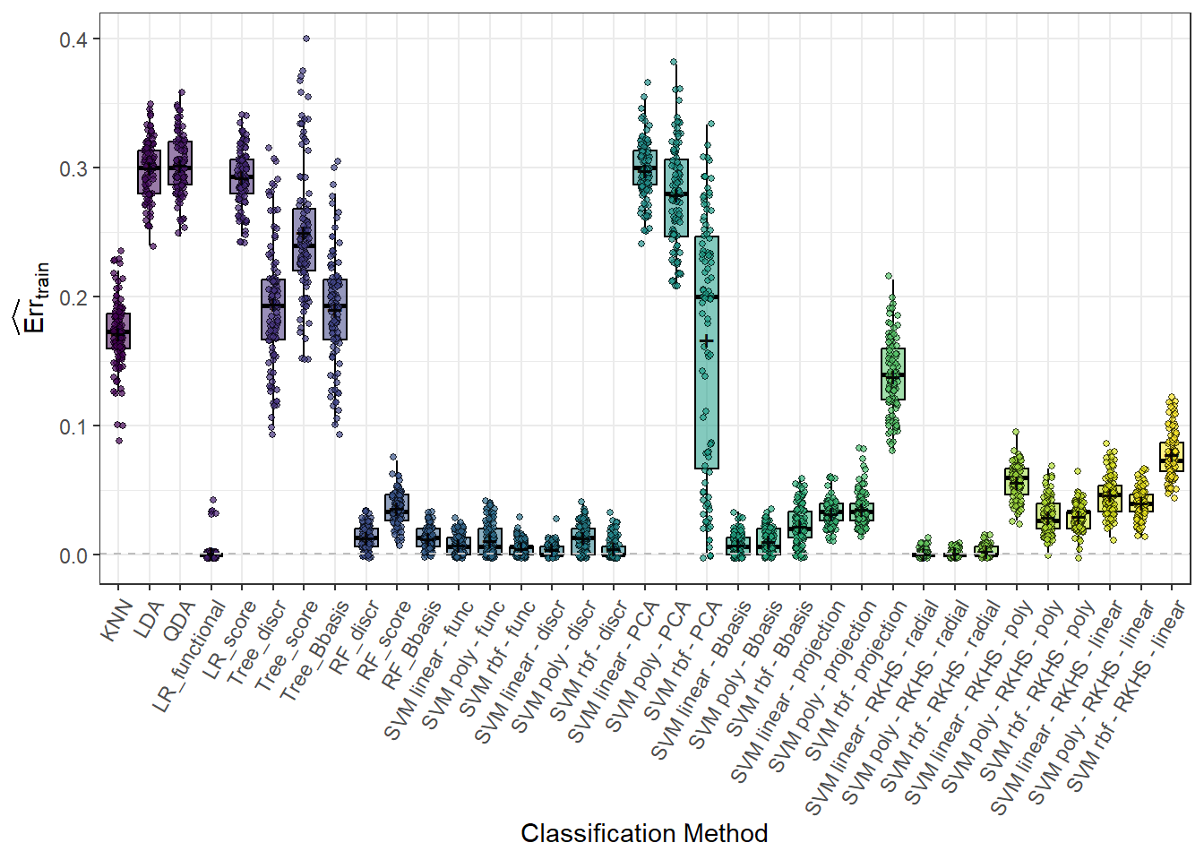 

Figure 6.18: Box plots of training error rates for 100 simulations separately for each classification method. The black symbols \(+\) denote the means.

Code

# for test data
SIMULACE$test |> 
  pivot_longer(cols = methods, names_to = 'method', values_to = 'Err') |>
  mutate(method = factor(method, levels = methods, labels = methods, ordered = TRUE)) |> 
  as.data.frame() |>
      filter(method %in% sub_methods) |>
  ggplot(aes(x = method, y = Err, fill = method, colour = method, alpha = method)) + 
    geom_jitter(position = position_jitter(height = 0, width = 0.15), alpha = 0.6, size = 0.9, pch = 21,
              colour = "black") +
  geom_boxplot(outlier.colour = "white", outlier.shape = 16, outlier.size = 0, 
               notch = FALSE, colour = 'black') + 
  theme_bw() + 
  labs(x = 'Classification Method',
       y = "$\\widehat{\\textnormal{Err}}_{test}$"
       # y = expression(widehat(Err)[test])
       ) + 
  theme(legend.position = 'none',
        axis.text.x = element_text(angle = 45, hjust = 1)) +
  stat_summary(fun = "mean", geom = "point", shape = 4,
               size = 2, color = "black", alpha = 1) +
  scale_x_discrete(labels = methods_names1) +
  theme(plot.margin = unit(c(0.1, 0.1, 0.7, 0.5), "cm")) +
  scale_fill_manual(values = box_col1) +
  scale_alpha_manual(values = box_alpha1) +
  geom_hline(yintercept = min(SIMULACE.df$Err.test), 
             linetype = 'dashed', colour = 'gray25', alpha = 0.8)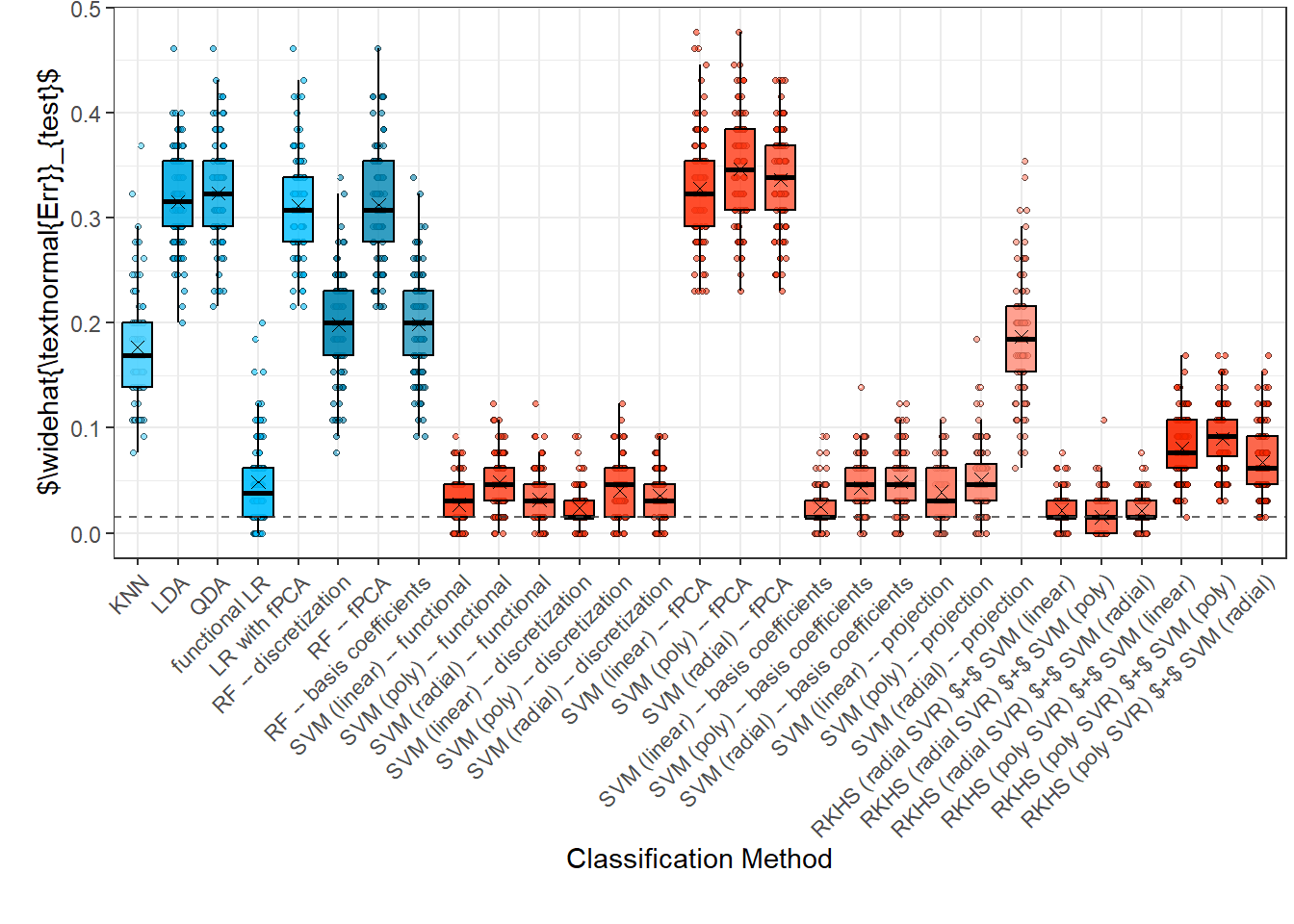

Figure 6.19: Box plots of test error rates for 100 simulations separately for each classification method. The black symbols \(+\) denote the means.

Code

# ggsave("figures/results_tec_neder.tex", device = tikz, width = 7, height = 5)
# ggsave("figures/kap7_tecator_box_test_neder_subset.tex", device = tikz, width = 6.5, height = 5)

Finally, let’s take a look at which hyperparameter values were the most frequently chosen.

Table 6.18: Medians of hyperparameter values for selected methods where some hyperparameter was determined using cross-validation.

	Median Hyperparameter Value
KNN_K	1.0
nharm	1.0
LR_func_n_basis	10.0
SVM_d_Linear	6.0
SVM_d_Poly	6.0
SVM_d_Radial	6.0
SVM_RKHS_radial_gamma1	3.7
SVM_RKHS_radial_gamma2	1.0
SVM_RKHS_radial_gamma3	1.0
SVM_RKHS_radial_d1	16.0
SVM_RKHS_radial_d2	16.0
SVM_RKHS_radial_d3	20.0
SVM_RKHS_poly_p1	4.0
SVM_RKHS_poly_p2	5.0
SVM_RKHS_poly_p3	5.0
SVM_RKHS_poly_d1	8.0
SVM_RKHS_poly_d2	6.0
SVM_RKHS_poly_d3	7.0
SVM_RKHS_linear_d1	17.0
SVM_RKHS_linear_d2	17.0
SVM_RKHS_linear_d3	13.0

Code

CV_res <- CV_RESULTS |> 
  pivot_longer(cols = CV_RESULTS |> colnames(), names_to = 'method', values_to = 'hyperparameter') |>
  mutate(method = factor(method, 
                         levels = CV_RESULTS |> colnames(), 
                         labels = CV_RESULTS |> colnames(), ordered = TRUE)) |> 
  as.data.frame() 

CV_res |> 
  filter(method %in% c('KNN_K', 'nharm', 'LR_func_n_basis')) |>
  ggplot(aes(x = hyperparameter, #y = after_stat(density),
             fill = method, colour = method)) + 
  geom_histogram(binwidth = 1, alpha = 0.6) + 
  theme_bw() + 
  facet_grid(~method, scales = 'free') +
  labs(x = 'Hyperparameter Values',
       y = 'Absolute Count') + 
  theme(legend.position = 'none')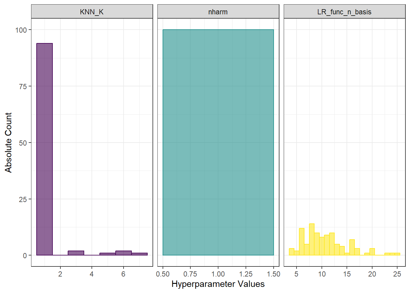

Figure 6.20: Histograms of hyperparameter values for KNN, functional logistic regression, and also a histogram for the number of principal components.

Code

CV_res |> 
  filter(method %in% c('SVM_d_Linear', 'SVM_d_Poly', 'SVM_d_Radial')) |>
  ggplot(aes(x = hyperparameter, #y = after_stat(density),
             fill = method, colour = method)) + 
  geom_histogram(binwidth = 1, alpha = 0.6) + 
  theme_bw() + 
  facet_grid(~method, scales = 'free') +
  labs(x = 'Hyperparameter Values',
       y = 'Absolute Count') + 
  theme(legend.position = 'none')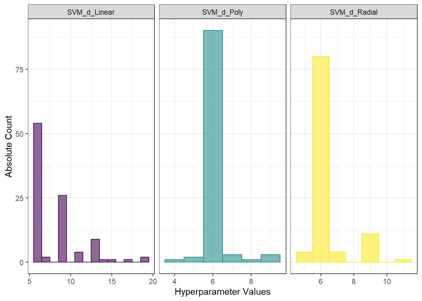

Figure 6.21: Histograms of hyperparameter values for SVM method with projection on B-spline basis.

Code

CV_res |> 
  filter(method %in% c('SVM_RKHS_radial_gamma1', 'SVM_RKHS_radial_gamma2',
                       'SVM_RKHS_radial_gamma3', 'SVM_RKHS_radial_d1', 
                       'SVM_RKHS_radial_d2', 'SVM_RKHS_radial_d3')) |>
  ggplot(aes(x = hyperparameter, #y = after_stat(density),
             fill = method, colour = method)) + 
  geom_histogram(bins = 10, alpha = 0.6) + 
  theme_bw() + 
  facet_wrap(~method, scales = 'free', ncol = 3) +
  labs(x = 'Hyperparameter Values',
       y = 'Absolute Count') + 
  theme(legend.position = 'none')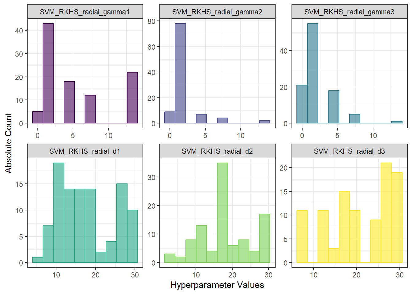

Figure 6.22: Histograms of hyperparameter values for RKHS + SVM with radial kernel.

Code

CV_res |> 
  filter(method %in% c('SVM_RKHS_poly_p1', 'SVM_RKHS_poly_p2',
                       'SVM_RKHS_poly_p3', 'SVM_RKHS_poly_d1',
                       'SVM_RKHS_poly_d2', 'SVM_RKHS_poly_d3')) |>
  ggplot(aes(x = hyperparameter, #y = after_stat(density),
             fill = method, colour = method)) + 
  geom_histogram(binwidth = 1, alpha = 0.6) + 
  theme_bw() + 
  facet_wrap(~method, scales = 'free', ncol = 3) +
  labs(x = 'Hyperparameter values',
       y = 'Absolute count') + 
  theme(legend.position = 'none')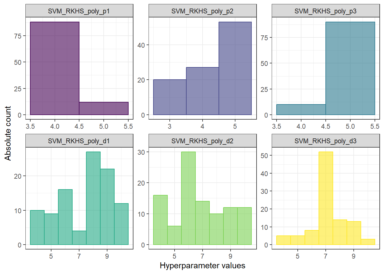

Figure 6.23: Histograms of hyperparameter values for the RKHS + SVM with polynomial kernel.

Code

CV_res |> 
  filter(method %in% c('SVM_RKHS_linear_d1',
                       'SVM_RKHS_linear_d2', 'SVM_RKHS_linear_d3')) |>
  ggplot(aes(x = hyperparameter, #y = after_stat(density),
             fill = method, colour = method)) + 
  geom_histogram(binwidth = 5, alpha = 0.6) + 
  theme_bw() + 
  facet_wrap(~method, scales = 'free', ncol = 3) +
  labs(x = 'Hyperparameter values',
       y = 'Absolute count') + 
  theme(legend.position = 'none')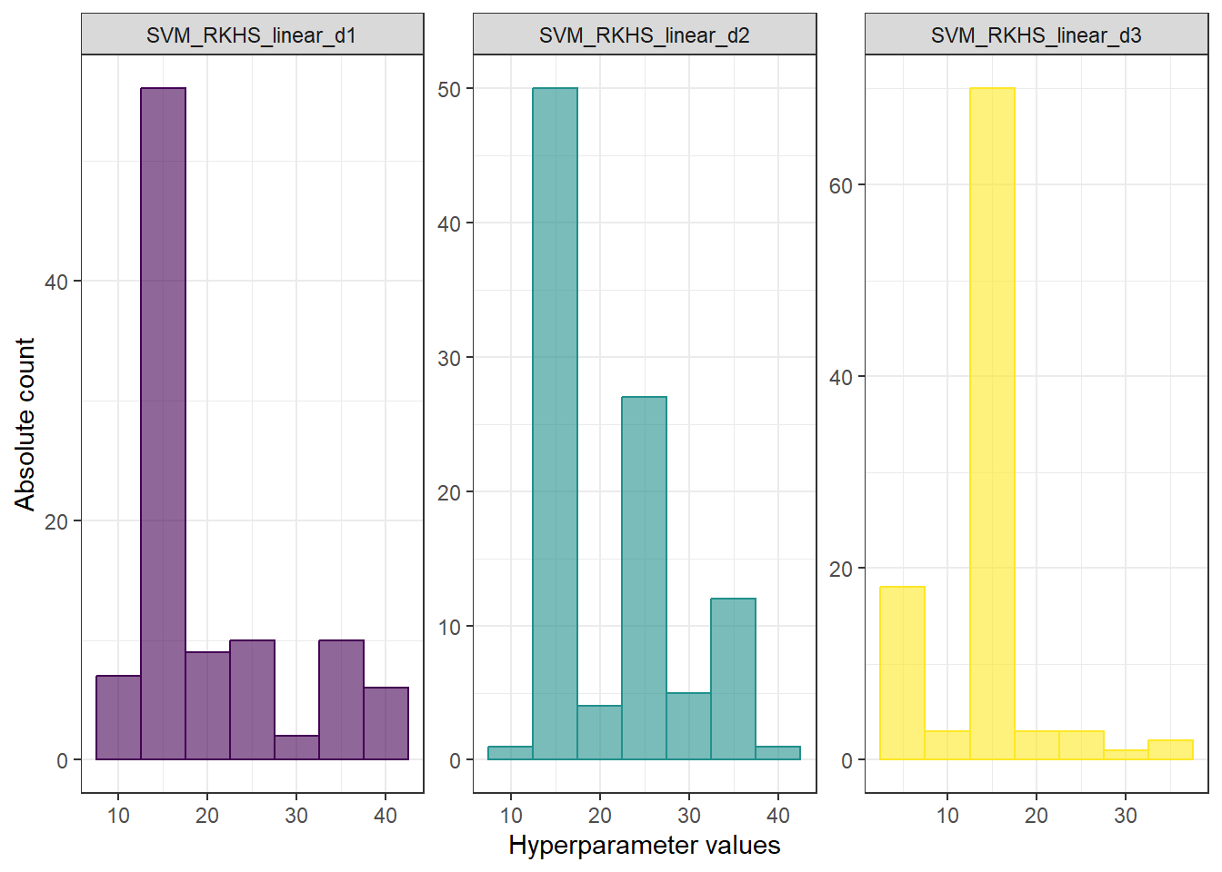

Figure 6.24: Histograms of hyperparameter values for the RKHS + SVM with linear kernel.

6.5.2 Simulation for derivations

Now let’s finally take a look at the simulation of derived data (we determined the second derivative of the curves).

Code

# Setting the random number generator
set.seed(41)

# Number of simulations
n.sim <- 100

## List to store error values
# Columns will represent methods
# Rows will represent individual repetitions
# List has two items ... train and test
methods <- c('KNN', 'LDA', 'QDA', 'LR_functional', 'LR_score', 'Tree_discr',
             'Tree_score', 'Tree_Bbasis', 'RF_discr', 'RF_score', 'RF_Bbasis',
             'SVM linear - func', 'SVM poly - func', 'SVM rbf - func',
             'SVM linear - diskr', 'SVM poly - diskr', 'SVM rbf - diskr', 
             'SVM linear - PCA', 'SVM poly - PCA', 'SVM rbf - PCA', 
             'SVM linear - Bbasis', 'SVM poly - Bbasis', 'SVM rbf - Bbasis',
             'SVM linear - projection', 'SVM poly - projection', 
             'SVM rbf - projection', 'SVM linear - RKHS - radial', 
             'SVM poly - RKHS - radial', 'SVM rbf - RKHS - radial', 
             'SVM linear - RKHS - poly', 'SVM poly - RKHS - poly', 
             'SVM rbf - RKHS - poly', 'SVM linear - RKHS - linear', 
             'SVM poly - RKHS - linear', 'SVM rbf - RKHS - linear')

SIMULACE <- list(train = as.data.frame(matrix(NA, ncol = length(methods), 
                                             nrow = n.sim,
                                             dimnames = list(1:n.sim, methods))), 
                 test = as.data.frame(matrix(NA, ncol = length(methods), 
                                             nrow = n.sim,
                                             dimnames = list(1:n.sim, methods))))

# Object to store optimal hyperparameter values determined using CV
CV_RESULTS <- data.frame(KNN_K = rep(NA, n.sim), 
                         nharm = NA, 
                         LR_func_n_basis = NA,
                         SVM_d_Linear = NA,
                         SVM_d_Poly = NA,
                         SVM_d_Radial = NA, 
                         SVM_RKHS_radial_gamma1 = NA,
                         SVM_RKHS_radial_gamma2 = NA,
                         SVM_RKHS_radial_gamma3 = NA,
                         SVM_RKHS_radial_d1 = NA,
                         SVM_RKHS_radial_d2 = NA,
                         SVM_RKHS_radial_d3 = NA,
                         SVM_RKHS_poly_p1 = NA,
                         SVM_RKHS_poly_p2 = NA,
                         SVM_RKHS_poly_p3 = NA,
                         SVM_RKHS_poly_d1 = NA,
                         SVM_RKHS_poly_d2 = NA,
                         SVM_RKHS_poly_d3 = NA,
                         SVM_RKHS_linear_d1 = NA,
                         SVM_RKHS_linear_d2 = NA,
                         SVM_RKHS_linear_d3 = NA)

Now we will repeat the entire previous section 100 times, storing the error values in the SIMULACE list. We will then store the optimal hyperparameter values in the CV_RESULTS data table—specifically for the \(K\)-nearest neighbors method and for SVM, the dimension \(d\) in the case of projection onto the B-spline basis. We will also save all hyperparameter values for the SVM + RKHS method.

Code

# nastaveni generatoru pseudonahodnych cisel
set.seed(41)

## SIMULACE

for(sim in 1:n.sim) {
  # rozdeleni na testovaci a trenovaci cast
  split <- sample.split(XXder$fdnames$reps, SplitRatio = 0.7)
  
  # vytvoreni vektoru 0 a 1, 0 pro < 20 a 1 pro > 20 
  Y <- ifelse(labels == 'large', 1, 0)
  
  X.train <- subset(XXder, split == TRUE)
  X.test <- subset(XXder, split == FALSE)
  
  Y.train <- subset(Y, split == TRUE)
  Y.test <- subset(Y, split == FALSE)
  
  x.train <- fdata(X.train)
  y.train <- as.numeric(factor(Y.train))
  
  ## 1) K nejbližších sousedů
  
  k_cv <- 10 # k-fold CV
  neighbours <- c(1:10) # pocet sousedu 
  
  # rozdelime trenovaci data na k casti
  folds <- createMultiFolds(X.train$fdnames$reps, k = k_cv, time = 1)
  
  # kontrola, ze mame opravdu k = k_cv
  while (length(folds) != k_cv) {
    folds <- createMultiFolds(X.train$fdnames$reps, k = k_cv, time = 1)
  }
  
  CV.results <- matrix(NA, nrow = length(neighbours), ncol = k_cv)
  
  for (index in 1:k_cv) {
    # definujeme danou indexovou mnozinu
    fold <- folds[[index]]
      
    x.train.cv <- subset(X.train, c(1:length(X.train$fdnames$reps)) %in% fold) |>
      fdata()
    y.train.cv <- subset(Y.train, c(1:length(X.train$fdnames$reps)) %in% fold) |>
      factor() |> as.numeric()
    
    x.test.cv <- subset(X.train, !c(1:length(X.train$fdnames$reps)) %in% fold) |>
      fdata()
    y.test.cv <- subset(Y.train, !c(1:length(X.train$fdnames$reps)) %in% fold) |>
      factor() |> as.numeric()
    
    # projdeme kazdou cast ... k-krat zopakujeme
    for(neighbour in neighbours) {
      # model pro konkretni volbu K
      neighb.model <- classif.knn(group = y.train.cv, 
                                fdataobj = x.train.cv, 
                                knn = neighbour) 
      # predikce na validacni casti
      model.neighb.predict <- predict(neighb.model, 
                                      new.fdataobj = x.test.cv)
      # presnost na validacni casti
      presnost <- table(y.test.cv, model.neighb.predict) |> 
        prop.table() |> diag() |> sum()
      
      # presnost vlozime na pozici pro dane K a fold
      CV.results[neighbour, index] <- presnost
    }
  }
  
  # spocitame prumerne presnosti pro jednotliva K pres folds
  CV.results <- apply(CV.results, 1, mean)
  K.opt <- which.max(CV.results)
  CV_RESULTS$KNN_K[sim] <- K.opt
  presnost.opt.cv <- max(CV.results)
  CV.results <- data.frame(K = neighbours, CV = CV.results)
  
  neighb.model <- classif.knn(group = y.train, fdataobj = x.train, knn = K.opt)
  
  # predikce
  model.neighb.predict <- predict(neighb.model, 
                                  new.fdataobj = fdata(X.test))
  
  presnost <- table(as.numeric(factor(Y.test)), model.neighb.predict) |>
    prop.table() |>
    diag() |>
    sum()
  
  RESULTS <- data.frame(model = 'KNN', 
                        Err.train = 1 - neighb.model$max.prob,
                        Err.test = 1 - presnost)
  
  ## 2) Lineární diskriminační analýza
  
  # analyza hlavnich komponent
  data.PCA <- pca.fd(X.train, nharm = 10) # nharm - maximalni pocet HK
  nharm <- which(cumsum(data.PCA$varprop) >= 0.9)[1] # urceni p
  CV_RESULTS$nharm[sim] <- nharm
  if(nharm == 1) nharm <- 2
  
  data.PCA <- pca.fd(X.train, nharm = nharm) 
  data.PCA.train <- as.data.frame(data.PCA$scores) # skore prvnich p HK
  data.PCA.train$Y <- factor(Y.train) # prislusnost do trid
  
  # vypocet skoru testovacich funkci
  scores <- matrix(NA, ncol = nharm, nrow = length(Y.test)) # prazdna matice 
  
  for(k in 1:dim(scores)[1]) {
    xfd = X.test[k] - data.PCA$meanfd[1] # k-te pozorovani - prumerna funkce
    scores[k, ] = inprod(xfd, data.PCA$harmonics) 
    # skalarni soucin rezidua a vlastnich funkci rho (funkcionalni hlavni komponenty)
  }
  
  data.PCA.test <- as.data.frame(scores)
  data.PCA.test$Y <- factor(Y.test)
  colnames(data.PCA.test) <- colnames(data.PCA.train) 
  
  # model
  clf.LDA <- lda(Y ~ ., data = data.PCA.train)
  
  # presnost na trenovacich datech
  predictions.train <- predict(clf.LDA, newdata = data.PCA.train)
  presnost.train <- table(data.PCA.train$Y, predictions.train$class) |>
    prop.table() |> diag() |> sum()
    
  # presnost na trenovacich datech
  predictions.test <- predict(clf.LDA, newdata = data.PCA.test)
  presnost.test <- table(data.PCA.test$Y, predictions.test$class) |>
    prop.table() |> diag() |> sum()
  
  Res <- data.frame(model = 'LDA', 
                    Err.train = 1 - presnost.train,
                    Err.test = 1 - presnost.test)
  
  RESULTS <- rbind(RESULTS, Res)
  
  ## 3) Kvadratická diskriminační analýza
  
  # model
  clf.QDA <- qda(Y ~ ., data = data.PCA.train)
  
  # presnost na trenovacich datech
  predictions.train <- predict(clf.QDA, newdata = data.PCA.train)
  presnost.train <- table(data.PCA.train$Y, predictions.train$class) |>
    prop.table() |> diag() |> sum()
    
  # presnost na trenovacich datech
  predictions.test <- predict(clf.QDA, newdata = data.PCA.test)
  presnost.test <- table(data.PCA.test$Y, predictions.test$class) |>
    prop.table() |> diag() |> sum()
  
  Res <- data.frame(model = 'QDA', 
                    Err.train = 1 - presnost.train,
                    Err.test = 1 - presnost.test)
  
  RESULTS <- rbind(RESULTS, Res)
  
  ## 4) Logistická regrese
  ### 4.1) Funkcionální logistická regrese
  
  # vytvorime vhodne objekty
  x.train <- fdata(X.train)
  y.train <- as.numeric(Y.train)
  
  # body, ve kterych jsou funkce vyhodnoceny
  tt <- x.train[["argvals"]]
  
  dataf <- as.data.frame(y.train) 
  colnames(dataf) <- "Y"
  # B-spline baze 
  nbasis.x <- 100
  basis1 <- create.bspline.basis(rangeval = range(tt), 
                                 nbasis = nbasis.x)
  
  ### 10-fold cross-validation
  n.basis.max <- 25
  n.basis <- 4:n.basis.max
  k_cv <- 10 # k-fold CV
  # rozdelime trenovaci data na k casti
  folds <- createMultiFolds(X.train$fdnames$reps, k = k_cv, time = 1)
  # kontrola, ze mame opravdu k = k_cv
  while (length(folds) != k_cv) {
    folds <- createMultiFolds(X.train$fdnames$reps, k = k_cv, time = 1)
  }
  ## prvky, ktere se behem cyklu nemeni
  # body, ve kterych jsou funkce vyhodnoceny
  tt <- x.train[["argvals"]]
  rangeval <- range(tt)
  # vztah
  f <- Y ~ x
  # baze pro x
  basis.x <- list("x" = basis1)
  
  CV.results <- matrix(NA, nrow = length(n.basis), ncol = k_cv, 
                       dimnames = list(n.basis, 1:k_cv))
  
  for (index in 1:k_cv) {
    # definujeme danou indexovou mnozinu
    fold <- folds[[index]]
      
    x.train.cv <- subset(X.train, c(1:length(X.train$fdnames$reps)) %in% fold) |>
      fdata()
    y.train.cv <- subset(Y.train, c(1:length(X.train$fdnames$reps)) %in% fold) |>
      as.numeric()
    
    x.test.cv <- subset(X.train, !c(1:length(X.train$fdnames$reps)) %in% fold) |>
      fdata()
    y.test.cv <- subset(Y.train, !c(1:length(X.train$fdnames$reps)) %in% fold) |>
      as.numeric()
    
    dataf <- as.data.frame(y.train.cv) 
    colnames(dataf) <- "Y"
    
    for (i in n.basis) {
      # baze pro bety
      basis2 <- create.bspline.basis(rangeval = rangeval, nbasis = i)
      
      basis.b <- list("x" = basis2)
      # vstupni data do modelu
      ldata <- list("df" = dataf, "x" = x.train.cv)
      # binomicky model ... model logisticke regrese
      model.glm <- fregre.glm(f, family = binomial(), data = ldata,
                              basis.x = basis.x, basis.b = basis.b)
      
      # presnost na validacni casti 
      newldata = list("df" = as.data.frame(y.test.cv), "x" = x.test.cv)
      predictions.valid <- predict(model.glm, newx = newldata)
      predictions.valid <- data.frame(Y.pred = ifelse(predictions.valid < 1/2, 0, 1))
      presnost.valid <- table(y.test.cv, predictions.valid$Y.pred) |>
        prop.table() |> diag() |> sum()
      
      # vlozime do matice
      CV.results[as.character(i), as.character(index)] <- presnost.valid
    } 
  }
  
  # spocitame prumerne presnosti pro jednotliva n pres folds
  CV.results <- apply(CV.results, 1, mean)
  n.basis.opt <- n.basis[which.max(CV.results)]
  CV_RESULTS$LR_func_n_basis[sim] <- n.basis.opt
  presnost.opt.cv <- max(CV.results)
  
  # optimalni model
  basis2 <- create.bspline.basis(rangeval = range(tt), nbasis = n.basis.opt)
  f <- Y ~ x
  # baze pro x a bety
  basis.x <- list("x" = basis1) 
  basis.b <- list("x" = basis2)
  # vstupni data do modelu
  dataf <- as.data.frame(y.train) 
  colnames(dataf) <- "Y"
  ldata <- list("df" = dataf, "x" = x.train)
  # binomicky model ... model logisticke regrese
  model.glm <- fregre.glm(f, family = binomial(), data = ldata,
                          basis.x = basis.x, basis.b = basis.b)
  
  # presnost na trenovacich datech
  predictions.train <- predict(model.glm, newx = ldata)
  predictions.train <- data.frame(Y.pred = ifelse(predictions.train < 1/2, 0, 1))
  presnost.train <- table(Y.train, predictions.train$Y.pred) |>
    prop.table() |> diag() |> sum()
    
  # presnost na trenovacich datech
  newldata = list("df" = as.data.frame(Y.test), "x" = fdata(X.test))
  predictions.test <- predict(model.glm, newx = newldata)
  predictions.test <- data.frame(Y.pred = ifelse(predictions.test < 1/2, 0, 1))
  presnost.test <- table(Y.test, predictions.test$Y.pred) |>
    prop.table() |> diag() |> sum()
  
  Res <- data.frame(model = 'LR_functional', 
                    Err.train = 1 - presnost.train,
                    Err.test = 1 - presnost.test)
  
  RESULTS <- rbind(RESULTS, Res)
  
  ### 4.2) Logistická regrese s analýzou hlavních komponent
  
  # model
  clf.LR <- glm(Y ~  ., data = data.PCA.train, family = binomial)
  
  # presnost na trenovacich datech
  predictions.train <- predict(clf.LR, newdata = data.PCA.train, type = 'response')
  predictions.train <- ifelse(predictions.train > 0.5, 1, 0)
  presnost.train <- table(data.PCA.train$Y, predictions.train) |>
    prop.table() |> diag() |> sum()
    
  # presnost na trenovacich datech
  predictions.test <- predict(clf.LR, newdata = data.PCA.test, type = 'response')
  predictions.test <- ifelse(predictions.test > 0.5, 1, 0)
  presnost.test <- table(data.PCA.test$Y, predictions.test) |>
    prop.table() |> diag() |> sum()
  
  Res <- data.frame(model = 'LR_score', 
                    Err.train = 1 - presnost.train,
                    Err.test = 1 - presnost.test)
  
  RESULTS <- rbind(RESULTS, Res)
  
  ## 5) Rozhodovací stromy
  ### 5.1) Diskretizace intervalu
  
  # posloupnost bodu, ve kterych funkce vyhodnotime
  t.seq <- seq(min(t), max(t), length = 101)
     
  grid.data <- eval.fd(fdobj = X.train, evalarg = t.seq)
  grid.data <- as.data.frame(t(grid.data)) # transpozice kvuli funkcim v radku
  grid.data$Y <- Y.train |> factor()
  
  grid.data.test <- eval.fd(fdobj = X.test, evalarg = t.seq)
  grid.data.test <- as.data.frame(t(grid.data.test))
  grid.data.test$Y <- Y.test |> factor()
  
  # sestrojeni modelu
  clf.tree <- train(Y ~ ., data = grid.data, 
                   method = "rpart", 
                   trControl = trainControl(method = "CV", number = 10),
                   metric = "Accuracy")
  
  # presnost na trenovacich datech
  predictions.train <- predict(clf.tree, newdata = grid.data)
  presnost.train <- table(Y.train, predictions.train) |>
    prop.table() |> diag() |> sum()
    
  # presnost na trenovacich datech
  predictions.test <- predict(clf.tree, newdata = grid.data.test)
  presnost.test <- table(Y.test, predictions.test) |>
    prop.table() |> diag() |> sum()
  
  Res <- data.frame(model = 'Tree_discr', 
                    Err.train = 1 - presnost.train,
                    Err.test = 1 - presnost.test)
  
  RESULTS <- rbind(RESULTS, Res)
  
  ### 5.2) Skóre hlavních komponent
  
  # sestrojeni modelu
  clf.tree.PCA <- train(Y ~ ., data = data.PCA.train, 
                   method = "rpart", 
                   trControl = trainControl(method = "CV", number = 10),
                   metric = "Accuracy")
  
  # presnost na trenovacich datech
  predictions.train <- predict(clf.tree.PCA, newdata = data.PCA.train)
  presnost.train <- table(Y.train, predictions.train) |>
    prop.table() |> diag() |> sum()
    
  # presnost na trenovacich datech
  predictions.test <- predict(clf.tree.PCA, newdata = data.PCA.test)
  presnost.test <- table(Y.test, predictions.test) |>
    prop.table() |> diag() |> sum()
  
  Res <- data.frame(model = 'Tree_score', 
                    Err.train = 1 - presnost.train,
                    Err.test = 1 - presnost.test)
  
  RESULTS <- rbind(RESULTS, Res)
  
  ### 5.3) Bázové koeficienty
  
  # trenovaci dataset
  data.Bbasis.train <- t(X.train$coefs) |> as.data.frame()
  data.Bbasis.train$Y <- factor(Y.train)
  
  # testovaci dataset
  data.Bbasis.test <- t(X.test$coefs) |> as.data.frame()
  data.Bbasis.test$Y <- factor(Y.test)
  
  # sestrojeni modelu
  clf.tree.Bbasis <- train(Y ~ ., data = data.Bbasis.train, 
                   method = "rpart", 
                   trControl = trainControl(method = "CV", number = 10),
                   metric = "Accuracy")
  
  # presnost na trenovacich datech
  predictions.train <- predict(clf.tree.Bbasis, newdata = data.Bbasis.train)
  presnost.train <- table(Y.train, predictions.train) |>
    prop.table() |> diag() |> sum()
    
  # presnost na trenovacich datech
  predictions.test <- predict(clf.tree.Bbasis, newdata = data.Bbasis.test)
  presnost.test <- table(Y.test, predictions.test) |>
    prop.table() |> diag() |> sum()
  
  Res <- data.frame(model = 'Tree_Bbasis', 
                    Err.train = 1 - presnost.train,
                    Err.test = 1 - presnost.test)
  
  RESULTS <- rbind(RESULTS, Res)
  
  ## 6) Náhodné lesy
  
  ### 6.1) Diskretizace intervalu
  
  # sestrojeni modelu
  clf.RF <- randomForest(Y ~ ., data = grid.data, 
                         ntree = 500, # pocet stromu
                         importance = TRUE,
                         nodesize = 5)
  
  # presnost na trenovacich datech
  predictions.train <- predict(clf.RF, newdata = grid.data)
  presnost.train <- table(Y.train, predictions.train) |>
    prop.table() |> diag() |> sum()
    
  # presnost na trenovacich datech
  predictions.test <- predict(clf.RF, newdata = grid.data.test)
  presnost.test <- table(Y.test, predictions.test) |>
    prop.table() |> diag() |> sum()
  
  Res <- data.frame(model = 'RF_discr', 
                    Err.train = 1 - presnost.train,
                    Err.test = 1 - presnost.test)
  
  RESULTS <- rbind(RESULTS, Res)
  
  ### 6.2) Skóre hlavních komponent
  
  # sestrojeni modelu
  clf.RF.PCA <- randomForest(Y ~ ., data = data.PCA.train, 
                             ntree = 500, # pocet stromu
                             importance = TRUE,
                             nodesize = 5)
  
  # presnost na trenovacich datech
  predictions.train <- predict(clf.RF.PCA, newdata = data.PCA.train)
  presnost.train <- table(Y.train, predictions.train) |>
    prop.table() |> diag() |> sum()
    
  # presnost na trenovacich datech
  predictions.test <- predict(clf.RF.PCA, newdata = data.PCA.test)
  presnost.test <- table(Y.test, predictions.test) |>
    prop.table() |> diag() |> sum()
  
  Res <- data.frame(model = 'RF_score', 
                    Err.train = 1 - presnost.train,
                    Err.test = 1 - presnost.test)
  
  RESULTS <- rbind(RESULTS, Res)
  
  ### 6.3) Bázové koeficienty
  
  # sestrojeni modelu
  clf.RF.Bbasis <- randomForest(Y ~ ., data = data.Bbasis.train, 
                                ntree = 500, # pocet stromu
                                importance = TRUE,
                                nodesize = 5)
  
  # presnost na trenovacich datech
  predictions.train <- predict(clf.RF.Bbasis, newdata = data.Bbasis.train)
  presnost.train <- table(Y.train, predictions.train) |>
    prop.table() |> diag() |> sum()
    
  # presnost na trenovacich datech
  predictions.test <- predict(clf.RF.Bbasis, newdata = data.Bbasis.test)
  presnost.test <- table(Y.test, predictions.test) |>
    prop.table() |> diag() |> sum()
  
  Res <- data.frame(model = 'RF_Bbasis', 
                    Err.train = 1 - presnost.train,
                    Err.test = 1 - presnost.test)
  
  RESULTS <- rbind(RESULTS, Res)
  
  ## 7) SVM
  
  # rozdeleni na testovaci a trenovaci cast
  X.train_norm <- subset(XXfd_norm_der, split == TRUE)
  X.test_norm <- subset(XXfd_norm_der, split == FALSE)
  
  Y.train_norm <- subset(Y, split == TRUE)
  Y.test_norm <- subset(Y, split == FALSE)
  
  grid.data <- eval.fd(fdobj = X.train_norm, evalarg = t.seq)
  grid.data <- as.data.frame(t(grid.data)) 
  grid.data$Y <- Y.train_norm |> factor()
  
  grid.data.test <- eval.fd(fdobj = X.test_norm, evalarg = t.seq)
  grid.data.test <- as.data.frame(t(grid.data.test))
  grid.data.test$Y <- Y.test_norm |> factor()
  
  # rozdelime trenovaci data na k casti
  folds <- createMultiFolds(1:sum(split), k = k_cv, time = 1)
  # kontrola, ze mame opravdu k = k_cv
  while (length(folds) != k_cv) {
    folds <- createMultiFolds(1:sum(split), k = k_cv, time = 1)
  }
  
  ### 7.0) SVM for functional data
  
  # ktere hodnoty gamma chceme uvazovat
  gamma.cv <- 10^seq(-5, 0, length = 5)
  C.cv <- 10^seq(-2, 4, length = 5)
  p.cv <- 3
  coef0 <- 1
  
  # list se tremi slozkami ... array pro jednotlive jadra -> linear, poly, radial
  # prazdna matice, do ktere vlozime jednotlive vysledky
  # ve sloupcich budou hodnoty presnosti pro dane
  # v radcich budou hodnoty pro danou gamma a vrstvy odpovidaji folds
  CV.results <- list(
    SVM.l = array(NA, dim = c(length(C.cv), k_cv)),
    SVM.p = array(NA, dim = c(length(C.cv), length(p.cv), k_cv)),
    SVM.r = array(NA, dim = c(length(C.cv), length(gamma.cv), k_cv))
  )
  
  # nejprve projdeme hodnoty C
  for (cost in C.cv) {
    # projdeme jednotlive folds
    for (index_cv in 1:k_cv) {
      # definice testovaci a trenovaci casti pro CV
      fold <- folds[[index_cv]]
      cv_sample <- 1:dim(X.train_norm$coefs)[2] %in% fold
      
      x.train.cv <- fdata(subset(X.train_norm, cv_sample))
      x.test.cv <- fdata(subset(X.train_norm, !cv_sample))
      y.train.cv <- as.factor(subset(Y.train_norm, cv_sample))
      y.test.cv <- as.factor(subset(Y.train_norm, !cv_sample))
      
      # body, ve kterych jsou funkce vyhodnoceny
      tt <- x.train.cv[["argvals"]]
      
      dataf <- as.data.frame(y.train.cv) 
      colnames(dataf) <- "Y"
      # B-spline baze 
      basis1 <- create.bspline.basis(rangeval = range(tt), 
                                     norder = 4, nbasis = 100)
      # formula
      f <- Y ~ x 
      # baze pro x
      basis.x <- list("x" = basis1) 
      # vstupni data do modelu
      ldata <- list("df" = dataf, "x" = x.train.cv)
      
      ## LINEARNI JADRO
      # model SVM
      clf.svm.f_l <- classif.svm(formula = f,
                  data = ldata,
                  basis.x = basis.x,
                  kernel = 'linear',
                  cost = cost,
                  type = 'C-classification',
                  scale = TRUE)
        
      # presnost na testovacich datech
      newdat <- list("x" = x.test.cv)
      predictions.test <- predict(clf.svm.f_l, newdat, type = 'class')
      presnost.test.l <- mean(y.test.cv == predictions.test)
      
      # presnosti vlozime na pozice pro dane C a fold
      CV.results$SVM.l[(1:length(C.cv))[C.cv == cost], 
                       index_cv] <- presnost.test.l
      
      ## POLYNOMIALNI JADRO
      for (p in p.cv) {
        # sestrojeni modelu
        clf.svm.f_p <- classif.svm(formula = f,
                  data = ldata,
                  basis.x = basis.x,
                  kernel = 'polynomial',
                  cost = cost,
                  coef0 = coef0,
                  degree = p,
                  type = 'C-classification',
                  scale = TRUE)
          
        # presnost na testovacich datech
        newdat <- list("x" = x.test.cv)
        predictions.test <- predict(clf.svm.f_p, newdat, type = 'class')
        presnost.test.p <- mean(y.test.cv == predictions.test)
        
        # presnosti vlozime na pozice pro dane C, p a fold
        CV.results$SVM.p[(1:length(C.cv))[C.cv == cost], 
                         (1:length(p.cv))[p.cv == p],
                         index_cv] <- presnost.test.p
      }
          
      ## RADIALNI JADRO
      for (gam.cv in gamma.cv) {
        # sestrojeni modelu
        clf.svm.f_r <- classif.svm(formula = f,
                  data = ldata,
                  basis.x = basis.x,
                  kernel = 'radial',
                  cost = cost,
                  gamma = gam.cv,
                  type = 'C-classification',
                  scale = TRUE)
          
        # presnost na testovacich datech
        newdat <- list("x" = x.test.cv)
        predictions.test <- predict(clf.svm.f_r, newdat, type = 'class')
        presnost.test.r <- mean(y.test.cv == predictions.test)
        
        # presnosti vlozime na pozice pro dane C, gamma a fold
        CV.results$SVM.r[(1:length(C.cv))[C.cv == cost], 
                         (1:length(gamma.cv))[gamma.cv == gam.cv],
                         index_cv] <- presnost.test.r
      }
    }
  }
  
  # spocitame prumerne presnosti pro jednotliva C pres folds
  ## Linearni jadro
  CV.results$SVM.l <- apply(CV.results$SVM.l, 1, mean)
  ## Polynomialni jadro
  CV.results$SVM.p <- apply(CV.results$SVM.p, c(1, 2), mean)
  ## Radialni jadro
  CV.results$SVM.r <- apply(CV.results$SVM.r, c(1, 2), mean)
  
  C.opt <- c(which.max(CV.results$SVM.l), 
             which.max(CV.results$SVM.p) %% length(C.cv), 
             which.max(CV.results$SVM.r) %% length(C.cv))
  C.opt[C.opt == 0] <- length(C.cv)
  C.opt <- C.cv[C.opt]
  
  gamma.opt <- which.max(t(CV.results$SVM.r)) %% length(gamma.cv)
  gamma.opt[gamma.opt == 0] <- length(gamma.cv)
  gamma.opt <- gamma.cv[gamma.opt]
  
  p.opt <- which.max(t(CV.results$SVM.p)) %% length(p.cv)
  p.opt[p.opt == 0] <- length(p.cv)
  p.opt <- p.cv[p.opt]
  
  presnost.opt.cv <- c(max(CV.results$SVM.l), 
                       max(CV.results$SVM.p),
                       max(CV.results$SVM.r))
  
  # vytvorime vhodne objekty
  x.train <- fdata(X.train_norm)
  y.train <- as.factor(Y.train_norm)
  
  # body, ve kterych jsou funkce vyhodnoceny
  tt <- x.train[["argvals"]]
  
  dataf <- as.data.frame(y.train) 
  colnames(dataf) <- "Y"
  # B-spline baze 
  # basis1 <- X.train_norm$basis
  
  # formula
  f <- Y ~ x 
  # baze pro x
  basis.x <- list("x" = basis1) 
  # vstupni data do modelu
  ldata <- list("df" = dataf, "x" = x.train)
  
  model.svm.f_l <- classif.svm(formula = f,
              data = ldata,
              basis.x = basis.x,
              kernel = 'linear', 
              type = 'C-classification',
              scale = TRUE,
              cost = C.opt[1])
  
  model.svm.f_p <- classif.svm(formula = f,
              data = ldata,
              basis.x = basis.x,
              kernel = 'polynomial', 
              type = 'C-classification',
              scale = TRUE,
              degree = p.opt,
              coef0 = coef0,
              cost = C.opt[2])
  
  model.svm.f_r <- classif.svm(formula = f,
              data = ldata,
              basis.x = basis.x,
              kernel = 'radial', 
              type = 'C-classification',
              scale = TRUE,
              gamma = gamma.opt,
              cost = C.opt[3])
  
  # presnost na trenovacich datech
  newdat <- list("x" = x.train)
  predictions.train.l <- predict(model.svm.f_l, newdat, type = 'class')
  presnost.train.l <- mean(factor(Y.train_norm) == predictions.train.l)
  
  predictions.train.p <- predict(model.svm.f_p, newdat, type = 'class')
  presnost.train.p <- mean(factor(Y.train_norm) == predictions.train.p)
  
  predictions.train.r <- predict(model.svm.f_r, newdat, type = 'class')
  presnost.train.r <- mean(factor(Y.train_norm) == predictions.train.r)
    
  # presnost na testovacich datech
  newdat <- list("x" = fdata(X.test_norm))
  predictions.test.l <- predict(model.svm.f_l, newdat, type = 'class')
  presnost.test.l <- mean(factor(Y.test_norm) == predictions.test.l)
  
  predictions.test.p <- predict(model.svm.f_p, newdat, type = 'class')
  presnost.test.p <- mean(factor(Y.test_norm) == predictions.test.p)
  
  predictions.test.r <- predict(model.svm.f_r, newdat, type = 'class')
  presnost.test.r <- mean(factor(Y.test_norm) == predictions.test.r)
  
  Res <- data.frame(model = c('SVM linear - func', 
                              'SVM poly - func', 
                              'SVM rbf - func'), 
                    Err.train = 1 - c(presnost.train.l, presnost.train.p, presnost.train.r),
                    Err.test = 1 - c(presnost.test.l, presnost.test.p, presnost.test.r))
  
  RESULTS <- rbind(RESULTS, Res)
  
  ### 7.1) Diskretizace intervalu
  
  # ktere hodnoty gamma chceme uvazovat
  gamma.cv <- 10^seq(-4, -1, length = 5)
  C.cv <- 10^seq(-4, 2, length = 5)
  p.cv <- 3
  coef0 <- 1
  
  # list se tremi slozkami ... array pro jednotlive jadra -> linear, poly, radial
  # prazdna matice, do ktere vlozime jednotlive vysledky
  # ve sloupcich budou hodnoty presnosti pro dane
  # v radcich budou hodnoty pro danou gamma a vrstvy odpovidaji folds
  CV.results <- list(
    SVM.l = array(NA, dim = c(length(C.cv), k_cv)),
    SVM.p = array(NA, dim = c(length(C.cv), length(p.cv), k_cv)),
    SVM.r = array(NA, dim = c(length(C.cv), length(gamma.cv), k_cv))
  )
  
  # nejprve projdeme hodnoty C
  for (C in C.cv) {
    # projdeme jednotlive folds
    for (index_cv in 1:k_cv) {
      # definice testovaci a trenovaci casti pro CV
      fold <- folds[[index_cv]]
      cv_sample <- 1:dim(grid.data)[1] %in% fold
      
      data.grid.train.cv <- as.data.frame(grid.data[cv_sample, ])
      data.grid.test.cv <- as.data.frame(grid.data[!cv_sample, ])
      
      ## LINEARNI JADRO
      # sestrojeni modelu
      clf.SVM.l <- svm(Y ~ ., data = data.grid.train.cv,
                       type = 'C-classification',
                       scale = TRUE,
                       cost = C,
                       kernel = 'linear')
      
      # presnost na validacnich datech
      predictions.test.l <- predict(clf.SVM.l, newdata = data.grid.test.cv)
      presnost.test.l <- table(data.grid.test.cv$Y, predictions.test.l) |>
        prop.table() |> diag() |> sum()
      
      # presnosti vlozime na pozice pro dane C a fold
      CV.results$SVM.l[(1:length(C.cv))[C.cv == C], 
                       index_cv] <- presnost.test.l
      
      ## POLYNOMIALNI JADRO
      for (p in p.cv) {
        # sestrojeni modelu
        clf.SVM.p <- svm(Y ~ ., data = data.grid.train.cv,
                         type = 'C-classification',
                         scale = TRUE,
                         cost = C,
                         coef0 = coef0,
                         degree = p,
                         kernel = 'polynomial')
        
        # presnost na validacnich datech
        predictions.test.p <- predict(clf.SVM.p, 
                                      newdata = data.grid.test.cv)
        presnost.test.p <- table(data.grid.test.cv$Y, predictions.test.p) |>
          prop.table() |> diag() |> sum()
        
        # presnosti vlozime na pozice pro dane C, p a fold
        CV.results$SVM.p[(1:length(C.cv))[C.cv == C], 
                         (1:length(p.cv))[p.cv == p],
                         index_cv] <- presnost.test.p
      }
          
      ## RADIALNI JADRO
      for (gamma in gamma.cv) {
        # sestrojeni modelu
        clf.SVM.r <- svm(Y ~ ., data = data.grid.train.cv,
                         type = 'C-classification',
                         scale = TRUE,
                         cost = C,
                         gamma = gamma,
                         kernel = 'radial')
        
        # presnost na validacnich datech
        predictions.test.r <- predict(clf.SVM.r, newdata = data.grid.test.cv)
        presnost.test.r <- table(data.grid.test.cv$Y, predictions.test.r) |>
          prop.table() |> diag() |> sum()
        
        # presnosti vlozime na pozice pro dane C, gamma a fold
        CV.results$SVM.r[(1:length(C.cv))[C.cv == C], 
                         (1:length(gamma.cv))[gamma.cv == gamma],
                         index_cv] <- presnost.test.r
      }
    }
  }
  # spocitame prumerne presnosti pro jednotliva C pres folds
  ## Linearni jadro
  CV.results$SVM.l <- apply(CV.results$SVM.l, 1, mean)
  ## Polynomialni jadro
  CV.results$SVM.p <- apply(CV.results$SVM.p, c(1, 2), mean)
  ## Radialni jadro
  CV.results$SVM.r <- apply(CV.results$SVM.r, c(1, 2), mean)
  
  C.opt <- c(which.max(CV.results$SVM.l), 
             which.max(CV.results$SVM.p) %% length(C.cv), 
             which.max(CV.results$SVM.r) %% length(C.cv))
  C.opt[C.opt == 0] <- length(C.cv)
  C.opt <- C.cv[C.opt]
  
  gamma.opt <- which.max(t(CV.results$SVM.r)) %% length(gamma.cv)
  gamma.opt[gamma.opt == 0] <- length(gamma.cv)
  gamma.opt <- gamma.cv[gamma.opt]
  
  p.opt <- which.max(t(CV.results$SVM.p)) %% length(p.cv)
  p.opt[p.opt == 0] <- length(p.cv)
  p.opt <- p.cv[p.opt]
  
  presnost.opt.cv <- c(max(CV.results$SVM.l), 
                       max(CV.results$SVM.p),
                       max(CV.results$SVM.r))
  
  # sestrojeni modelu
  clf.SVM.l <- svm(Y ~ ., data = grid.data,
                   type = 'C-classification',
                   scale = TRUE,
                   cost = C.opt[1],
                   kernel = 'linear')
  
  clf.SVM.p <- svm(Y ~ ., data = grid.data,
                   type = 'C-classification',
                   scale = TRUE,
                   cost = C.opt[2],
                   degree = p.opt,
                   coef0 = coef0,
                   kernel = 'polynomial')
  
  clf.SVM.r <- svm(Y ~ ., data = grid.data,
                   type = 'C-classification',
                   scale = TRUE, 
                   cost = C.opt[3],
                   gamma = gamma.opt,
                   kernel = 'radial')
  
  # presnost na trenovacich datech
  predictions.train.l <- predict(clf.SVM.l, newdata = grid.data)
  presnost.train.l <- table(Y.train, predictions.train.l) |>
    prop.table() |> diag() |> sum()
  
  predictions.train.p <- predict(clf.SVM.p, newdata = grid.data)
  presnost.train.p <- table(Y.train, predictions.train.p) |>
    prop.table() |> diag() |> sum()
  
  predictions.train.r <- predict(clf.SVM.r, newdata = grid.data)
  presnost.train.r <- table(Y.train, predictions.train.r) |>
    prop.table() |> diag() |> sum()
  
  # presnost na testovacich datech
  predictions.test.l <- predict(clf.SVM.l, newdata = grid.data.test)
  presnost.test.l <- table(Y.test, predictions.test.l) |>
    prop.table() |> diag() |> sum()
  
  predictions.test.p <- predict(clf.SVM.p, newdata = grid.data.test)
  presnost.test.p <- table(Y.test, predictions.test.p) |>
    prop.table() |> diag() |> sum()
  
  predictions.test.r <- predict(clf.SVM.r, newdata = grid.data.test)
  presnost.test.r <- table(Y.test, predictions.test.r) |>
    prop.table() |> diag() |> sum()
  
  Res <- data.frame(model = c('SVM linear - diskr', 
                              'SVM poly - diskr', 
                              'SVM rbf - diskr'), 
                    Err.train = 1 - c(presnost.train.l,
                                      presnost.train.p, presnost.train.r),
                    Err.test = 1 - c(presnost.test.l, 
                                     presnost.test.p, presnost.test.r))
  
  RESULTS <- rbind(RESULTS, Res)
  
  ### 7.2) Skóre hlavních komponent
  
  # ktere hodnoty gamma chceme uvazovat
  gamma.cv <- 10^seq(-2, 2, length = 5)
  C.cv <- 10^seq(-2, 5, length = 5)
  p.cv <- 3
  coef0 <- 1
  
  # list se tremi slozkami ... array pro jednotlive jadra -> linear, poly, radial
  # prazdna matice, do ktere vlozime jednotlive vysledky
  # ve sloupcich budou hodnoty presnosti pro dane
  # v radcich budou hodnoty pro danou gamma a vrstvy odpovidaji folds
  CV.results <- list(
    SVM.l = array(NA, dim = c(length(C.cv), k_cv)),
    SVM.p = array(NA, dim = c(length(C.cv), length(p.cv), k_cv)),
    SVM.r = array(NA, dim = c(length(C.cv), length(gamma.cv), k_cv))
  )
  
  # nejprve projdeme hodnoty C
  for (C in C.cv) {
    # projdeme jednotlive folds
    for (index_cv in 1:k_cv) {
      # definice testovaci a trenovaci casti pro CV
      fold <- folds[[index_cv]]
      cv_sample <- 1:dim(data.PCA.train)[1] %in% fold
      
      data.PCA.train.cv <- as.data.frame(data.PCA.train[cv_sample, ])
      data.PCA.test.cv <- as.data.frame(data.PCA.train[!cv_sample, ])
      
      ## LINEARNI JADRO
      # sestrojeni modelu
      clf.SVM.l <- svm(Y ~ ., data = data.PCA.train.cv,
                       type = 'C-classification',
                       scale = TRUE,
                       cost = C,
                       kernel = 'linear')
      
      # presnost na validacnich datech
      predictions.test.l <- predict(clf.SVM.l, newdata = data.PCA.test.cv)
      presnost.test.l <- table(data.PCA.test.cv$Y, predictions.test.l) |>
        prop.table() |> diag() |> sum()
      
      # presnosti vlozime na pozice pro dane C a fold
      CV.results$SVM.l[(1:length(C.cv))[C.cv == C], 
                       index_cv] <- presnost.test.l
      
      ## POLYNOMIALNI JADRO
      for (p in p.cv) {
        # sestrojeni modelu
        clf.SVM.p <- svm(Y ~ ., data = data.PCA.train.cv,
                         type = 'C-classification',
                         scale = TRUE,
                         cost = C,
                         coef0 = coef0,
                         degree = p,
                         kernel = 'polynomial')
        
        # presnost na validacnich datech
        predictions.test.p <- predict(clf.SVM.p, newdata = data.PCA.test.cv)
        presnost.test.p <- table(data.PCA.test.cv$Y, predictions.test.p) |>
          prop.table() |> diag() |> sum()
        
        # presnosti vlozime na pozice pro dane C, p a fold
        CV.results$SVM.p[(1:length(C.cv))[C.cv == C], 
                         (1:length(p.cv))[p.cv == p],
                         index_cv] <- presnost.test.p
      }
          
      ## RADIALNI JADRO
      for (gamma in gamma.cv) {
        # sestrojeni modelu
        clf.SVM.r <- svm(Y ~ ., data = data.PCA.train.cv,
                         type = 'C-classification',
                         scale = TRUE,
                         cost = C,
                         gamma = gamma,
                         kernel = 'radial')
        
        # presnost na validacnich datech
        predictions.test.r <- predict(clf.SVM.r, newdata = data.PCA.test.cv)
        presnost.test.r <- table(data.PCA.test.cv$Y, predictions.test.r) |>
          prop.table() |> diag() |> sum()
        
        # presnosti vlozime na pozice pro dane C, gamma a fold
        CV.results$SVM.r[(1:length(C.cv))[C.cv == C], 
                         (1:length(gamma.cv))[gamma.cv == gamma],
                         index_cv] <- presnost.test.r
      }
    }
  }
  # spocitame prumerne presnosti pro jednotliva C pres folds
  ## Linearni jadro
  CV.results$SVM.l <- apply(CV.results$SVM.l, 1, mean)
  ## Polynomialni jadro
  CV.results$SVM.p <- apply(CV.results$SVM.p, c(1, 2), mean)
  ## Radialni jadro
  CV.results$SVM.r <- apply(CV.results$SVM.r, c(1, 2), mean)
  
  C.opt <- c(which.max(CV.results$SVM.l), 
             which.max(CV.results$SVM.p) %% length(C.cv), 
             which.max(CV.results$SVM.r) %% length(C.cv))
  C.opt[C.opt == 0] <- length(C.cv)
  C.opt <- C.cv[C.opt]
  
  gamma.opt <- which.max(t(CV.results$SVM.r)) %% length(gamma.cv)
  gamma.opt[gamma.opt == 0] <- length(gamma.cv)
  gamma.opt <- gamma.cv[gamma.opt]
  
  p.opt <- which.max(t(CV.results$SVM.p)) %% length(p.cv)
  p.opt[p.opt == 0] <- length(p.cv)
  p.opt <- p.cv[p.opt]
  
  presnost.opt.cv <- c(max(CV.results$SVM.l), 
                       max(CV.results$SVM.p),
                       max(CV.results$SVM.r))
  # sestrojeni modelu
  clf.SVM.l.PCA <- svm(Y ~ ., data = data.PCA.train,
                       type = 'C-classification',
                       scale = TRUE,
                       cost = C.opt[1],
                       kernel = 'linear')
  
  clf.SVM.p.PCA <- svm(Y ~ ., data = data.PCA.train,
                       type = 'C-classification',
                       scale = TRUE,
                       cost = C.opt[2],
                       coef0 = coef0,
                       degree = p.opt,
                       kernel = 'polynomial')
  
  clf.SVM.r.PCA <- svm(Y ~ ., data = data.PCA.train,
                       type = 'C-classification',
                       scale = TRUE,
                       cost = C.opt[3],
                       gamma = gamma.opt,
                       kernel = 'radial')
  
  # presnost na trenovacich datech
  predictions.train.l <- predict(clf.SVM.l.PCA, newdata = data.PCA.train)
  presnost.train.l <- table(data.PCA.train$Y, predictions.train.l) |>
    prop.table() |> diag() |> sum()
  
  predictions.train.p <- predict(clf.SVM.p.PCA, newdata = data.PCA.train)
  presnost.train.p <- table(data.PCA.train$Y, predictions.train.p) |>
    prop.table() |> diag() |> sum()
  
  predictions.train.r <- predict(clf.SVM.r.PCA, newdata = data.PCA.train)
  presnost.train.r <- table(data.PCA.train$Y, predictions.train.r) |>
    prop.table() |> diag() |> sum()
    
  # presnost na testovacich datech
  predictions.test.l <- predict(clf.SVM.l.PCA, newdata = data.PCA.test)
  presnost.test.l <- table(data.PCA.test$Y, predictions.test.l) |>
    prop.table() |> diag() |> sum()
  
  predictions.test.p <- predict(clf.SVM.p.PCA, newdata = data.PCA.test)
  presnost.test.p <- table(data.PCA.test$Y, predictions.test.p) |>
    prop.table() |> diag() |> sum()
  
  predictions.test.r <- predict(clf.SVM.r.PCA, newdata = data.PCA.test)
  presnost.test.r <- table(data.PCA.test$Y, predictions.test.r) |>
    prop.table() |> diag() |> sum()
  
  Res <- data.frame(model = c('SVM linear - PCA', 
                              'SVM poly - PCA', 
                              'SVM rbf - PCA'), 
                    Err.train = 1 - c(presnost.train.l, 
                                      presnost.train.p, presnost.train.r),
                    Err.test = 1 - c(presnost.test.l, 
                                     presnost.test.p, presnost.test.r))
  
  RESULTS <- rbind(RESULTS, Res)
  
  ### 7.3) Bázové koeficienty
  
  # ktere hodnoty gamma chceme uvazovat
  gamma.cv <- 10^seq(-4, 0, length = 5)
  C.cv <- 10^seq(-4, 2, length = 5)
  p.cv <- 3
  coef0 <- 1
  
  # list se tremi slozkami ... array pro jednotlive jadra -> linear, poly, radial
  # prazdna matice, do ktere vlozime jednotlive vysledky
  # ve sloupcich budou hodnoty presnosti pro dane
  # v radcich budou hodnoty pro danou gamma a vrstvy odpovidaji folds
  CV.results <- list(
    SVM.l = array(NA, dim = c(length(C.cv), k_cv)),
    SVM.p = array(NA, dim = c(length(C.cv), length(p.cv), k_cv)),
    SVM.r = array(NA, dim = c(length(C.cv), length(gamma.cv), k_cv))
  )
  
  # nejprve projdeme hodnoty C
  for (C in C.cv) {
    # projdeme jednotlive folds
    for (index_cv in 1:k_cv) {
      # definice testovaci a trenovaci casti pro CV
      fold <- folds[[index_cv]]
      cv_sample <- 1:dim(grid.data)[1] %in% fold
      
      data.Bbasis.train.cv <- as.data.frame(data.Bbasis.train[cv_sample, ])
      data.Bbasis.test.cv <- as.data.frame(data.Bbasis.train[!cv_sample, ])
      
      ## LINEARNI JADRO
      # sestrojeni modelu
      clf.SVM.l <- svm(Y ~ ., data = data.Bbasis.train.cv,
                       type = 'C-classification',
                       scale = TRUE,
                       cost = C,
                       kernel = 'linear')
      
      # presnost na validacnich datech
      predictions.test.l <- predict(clf.SVM.l, newdata = data.Bbasis.test.cv)
      presnost.test.l <- table(data.Bbasis.test.cv$Y, predictions.test.l) |>
        prop.table() |> diag() |> sum()
      
      # presnosti vlozime na pozice pro dane C a fold
      CV.results$SVM.l[(1:length(C.cv))[C.cv == C], 
                       index_cv] <- presnost.test.l
      
      ## POLYNOMIALNI JADRO
      for (p in p.cv) {
        # sestrojeni modelu
        clf.SVM.p <- svm(Y ~ ., data = data.Bbasis.train.cv,
                         type = 'C-classification',
                         scale = TRUE,
                         cost = C,
                         coef0 = coef0,
                         degree = p,
                         kernel = 'polynomial')
        
        # presnost na validacnich datech
        predictions.test.p <- predict(clf.SVM.p, 
                                      newdata = data.Bbasis.test.cv)
        presnost.test.p <- table(data.Bbasis.test.cv$Y, predictions.test.p) |>
          prop.table() |> diag() |> sum()
        
        # presnosti vlozime na pozice pro dane C, p a fold
        CV.results$SVM.p[(1:length(C.cv))[C.cv == C], 
                         (1:length(p.cv))[p.cv == p],
                         index_cv] <- presnost.test.p
      }
          
      ## RADIALNI JADRO
      for (gamma in gamma.cv) {
        # sestrojeni modelu
        clf.SVM.r <- svm(Y ~ ., data = data.Bbasis.train.cv,
                         type = 'C-classification',
                         scale = TRUE,
                         cost = C,
                         gamma = gamma,
                         kernel = 'radial')
        
        # presnost na validacnich datech
        predictions.test.r <- predict(clf.SVM.r, 
                                      newdata = data.Bbasis.test.cv)
        presnost.test.r <- table(data.Bbasis.test.cv$Y, predictions.test.r) |>
          prop.table() |> diag() |> sum()
        
        # presnosti vlozime na pozice pro dane C, gamma a fold
        CV.results$SVM.r[(1:length(C.cv))[C.cv == C], 
                         (1:length(gamma.cv))[gamma.cv == gamma],
                         index_cv] <- presnost.test.r
      }
    }
  }
  # spocitame prumerne presnosti pro jednotliva C pres folds
  ## Linearni jadro
  CV.results$SVM.l <- apply(CV.results$SVM.l, 1, mean)
  ## Polynomialni jadro
  CV.results$SVM.p <- apply(CV.results$SVM.p, c(1, 2), mean)
  ## Radialni jadro
  CV.results$SVM.r <- apply(CV.results$SVM.r, c(1, 2), mean)
  
  C.opt <- c(which.max(CV.results$SVM.l), 
             which.max(CV.results$SVM.p) %% length(C.cv), 
             which.max(CV.results$SVM.r) %% length(C.cv))
  C.opt[C.opt == 0] <- length(C.cv)
  C.opt <- C.cv[C.opt]
  
  gamma.opt <- which.max(t(CV.results$SVM.r)) %% length(gamma.cv)
  gamma.opt[gamma.opt == 0] <- length(gamma.cv)
  gamma.opt <- gamma.cv[gamma.opt]
  
  p.opt <- which.max(t(CV.results$SVM.p)) %% length(p.cv)
  p.opt[p.opt == 0] <- length(p.cv)
  p.opt <- p.cv[p.opt]
  
  presnost.opt.cv <- c(max(CV.results$SVM.l), 
                       max(CV.results$SVM.p),
                       max(CV.results$SVM.r))
  # sestrojeni modelu
  clf.SVM.l.Bbasis <- svm(Y ~ ., data = data.Bbasis.train,
                          type = 'C-classification',
                          scale = TRUE,
                          cost = C.opt[1],
                          kernel = 'linear')
  
  clf.SVM.p.Bbasis <- svm(Y ~ ., data = data.Bbasis.train,
                          type = 'C-classification',
                          scale = TRUE,
                          cost = C.opt[2],
                          degree = p.opt,
                          coef0 = coef0,
                          kernel = 'polynomial')
  
  clf.SVM.r.Bbasis <- svm(Y ~ ., data = data.Bbasis.train,
                          type = 'C-classification',
                          scale = TRUE,
                          cost = C.opt[3],
                          gamma = gamma.opt,
                          kernel = 'radial')
  
  # presnost na trenovacich datech
  predictions.train.l <- predict(clf.SVM.l.Bbasis, newdata = data.Bbasis.train)
  presnost.train.l <- table(Y.train, predictions.train.l) |>
    prop.table() |> diag() |> sum()
  
  predictions.train.p <- predict(clf.SVM.p.Bbasis, newdata = data.Bbasis.train)
  presnost.train.p <- table(Y.train, predictions.train.p) |>
    prop.table() |> diag() |> sum()
  
  predictions.train.r <- predict(clf.SVM.r.Bbasis, newdata = data.Bbasis.train)
  presnost.train.r <- table(Y.train, predictions.train.r) |>
    prop.table() |> diag() |> sum()
    
  # presnost na testovacich datech
  predictions.test.l <- predict(clf.SVM.l.Bbasis, newdata = data.Bbasis.test)
  presnost.test.l <- table(Y.test, predictions.test.l) |>
    prop.table() |> diag() |> sum()
  
  predictions.test.p <- predict(clf.SVM.p.Bbasis, newdata = data.Bbasis.test)
  presnost.test.p <- table(Y.test, predictions.test.p) |>
    prop.table() |> diag() |> sum()
  
  predictions.test.r <- predict(clf.SVM.r.Bbasis, newdata = data.Bbasis.test)
  presnost.test.r <- table(Y.test, predictions.test.r) |>
    prop.table() |> diag() |> sum()

  Res <- data.frame(model = c('SVM linear - Bbasis', 
                              'SVM poly - Bbasis', 
                              'SVM rbf - Bbasis'), 
                    Err.train = 1 - c(presnost.train.l, 
                                      presnost.train.p, presnost.train.r),
                    Err.test = 1 - c(presnost.test.l, 
                                     presnost.test.p, presnost.test.r))

  RESULTS <- rbind(RESULTS, Res)
  
  ### 7.4) Projekce na B-splinovou bázi
  
  # hodnoty pro B-splinovou bazi
  rangeval <- range(t)
  norder <- 4
  n_basis_min <- norder
  n_basis_max <- 20
  dimensions <- n_basis_min:n_basis_max 
  folds <- createMultiFolds(1:sum(split), k = k_cv, time = 1)
  
  CV.results <- list(SVM.l = matrix(NA, nrow = length(dimensions), ncol = k_cv),
                     SVM.p = matrix(NA, nrow = length(dimensions), ncol = k_cv),
                     SVM.r = matrix(NA, nrow = length(dimensions), ncol = k_cv))
  
  for (d in dimensions) {
    bbasis <- create.bspline.basis(rangeval = rangeval, 
                                   nbasis = d)
    Projection <- project.basis(y = XX, argvals = t, basisobj = bbasis) 
    XX.train <- subset(t(Projection), split == TRUE)
    
    for (index_cv in 1:k_cv) {
      fold <- folds[[index_cv]]
      cv_sample <- 1:dim(XX.train)[1] %in% fold
      
      data.projection.train.cv <- as.data.frame(XX.train[cv_sample, ])
      data.projection.train.cv$Y <- factor(Y.train[cv_sample])
      data.projection.test.cv <- as.data.frame(XX.train[!cv_sample, ])
      Y.test.cv <- Y.train[!cv_sample]
      data.projection.test.cv$Y <- factor(Y.test.cv)
      # sestrojeni modelu
      clf.SVM.l.projection <- svm(Y ~ ., data = data.projection.train.cv,
                              type = 'C-classification',
                              scale = TRUE,
                              kernel = 'linear')
      
      clf.SVM.p.projection <- svm(Y ~ ., data = data.projection.train.cv,
                              type = 'C-classification',
                              scale = TRUE,
                              coef0 = coef0,
                              kernel = 'polynomial')
      
      clf.SVM.r.projection <- svm(Y ~ ., data = data.projection.train.cv,
                              type = 'C-classification',
                              scale = TRUE,
                              kernel = 'radial')
      # presnost na validacnich datech
      ## linear kernel
      predictions.test.l <- predict(clf.SVM.l.projection,
                                    newdata = data.projection.test.cv)
      presnost.test.l <- table(Y.test.cv, predictions.test.l) |>
        prop.table() |> diag() |> sum()
      ## polynomial kernel
      predictions.test.p <- predict(clf.SVM.p.projection, 
                                    newdata = data.projection.test.cv)
      presnost.test.p <- table(Y.test.cv, predictions.test.p) |>
        prop.table() |> diag() |> sum()
      ## radial kernel
      predictions.test.r <- predict(clf.SVM.r.projection,
                                    newdata = data.projection.test.cv)
      presnost.test.r <- table(Y.test.cv, predictions.test.r) |>
        prop.table() |> diag() |> sum()
      
      # presnosti vlozime na pozice pro dane d a fold
      CV.results$SVM.l[d - min(dimensions) + 1, index_cv] <- presnost.test.l
      CV.results$SVM.p[d - min(dimensions) + 1, index_cv] <- presnost.test.p
      CV.results$SVM.r[d - min(dimensions) + 1, index_cv] <- presnost.test.r
    }
  }
  
  # spocitame prumerne presnosti pro jednotliva d pres folds
  for (n_method in 1:length(CV.results)) {
    CV.results[[n_method]] <- apply(CV.results[[n_method]], 1, mean)
  }
  
  d.opt <- c(which.max(CV.results$SVM.l) + n_basis_min - 1, 
             which.max(CV.results$SVM.p) + n_basis_min - 1, 
             which.max(CV.results$SVM.r) + n_basis_min - 1)
  
  # ulozime optimalni d do datove tabulky
  CV_RESULTS[sim, 4:6] <- d.opt
  
  # pripravime si datovou tabulku pro ulozeni vysledku
  Res <- data.frame(model = c('SVM linear - projection', 
                              'SVM poly - projection', 
                              'SVM rbf - projection'), 
                    Err.train = NA,
                    Err.test = NA)
  
  for (kernel_number in 1:3) {
    kernel_type <- c('linear', 'polynomial', 'radial')[kernel_number]
    bbasis <- create.bspline.basis(rangeval = rangeval, 
                                   nbasis = d.opt[kernel_number])
    Projection <- project.basis(y = XX, argvals = t, basisobj = bbasis) 
    
    XX.train <- subset(t(Projection), split == TRUE)
    XX.test <- subset(t(Projection), split == FALSE)
    
    data.projection.train <- as.data.frame(XX.train)
    data.projection.train$Y <- factor(Y.train)
    
    data.projection.test <- as.data.frame(XX.test)
    data.projection.test$Y <- factor(Y.test)
    
    # sestrojeni modelu
    clf.SVM.projection <- svm(Y ~ ., data = data.projection.train,
                              type = 'C-classification',
                              scale = TRUE,
                              coef0 = coef0,
                              kernel = kernel_type)
    
    # presnost na trenovacich datech
    predictions.train <- predict(clf.SVM.projection, newdata = data.projection.train)
    presnost.train <- table(Y.train, predictions.train) |>
      prop.table() |> diag() |> sum()
      
    # presnost na trenovacich datech
    predictions.test <- predict(clf.SVM.projection, newdata = data.projection.test)
    presnost.test <- table(Y.test, predictions.test) |>
      prop.table() |> diag() |> sum()
    
    # ulozeni vysledku
    Res[kernel_number, c(2, 3)] <- 1 - c(presnost.train, presnost.test)
  }
  
  RESULTS <- rbind(RESULTS, Res)
  
  ## 7.5) SVM + RKHS
  
  C <- 1
  eps <- 0.01
  
  ### Gaussovo jadro
  
  # jadro a jadrova matice ... Gaussovske s parametrem gamma
  Gauss.kernel <- function(x, y, gamma) {
    return(exp(-gamma * norm(c(x - y) |> t(), type = 'F')))
  }
  
  Kernel.RKHS <- function(x, gamma) {
    K <- matrix(NA, ncol = length(x), nrow = length(x))
    for(i in 1:nrow(K)) {
      for(j in 1:ncol(K)) {
        K[i, j] <- Gauss.kernel(x = x[i], y = x[j], gamma = gamma)
      }
    }
    return(K)
  }
  
  # rozdelime trenovaci data na k casti
  folds <- createMultiFolds(1:sum(split), k = k_cv, time = 1)
  # odstranime posledni sloupec, ve kterem jsou hodnoty Y
  data.RKHS <- grid.data[, -dim(grid.data)[2]] |> t()
  
  # hodnoty hyperparametru, ktere budeme prochazet
  dimensions <- seq(2, 30, by = 2) # rozumny rozsah hodnot d
  gamma.cv <- 10^seq(-2, 2, length = 15)
  
  # list se tremi slozkami ... array pro jednotlive jadra -> linear, poly, radial
  # prazdna matice, do ktere vlozime jednotlive vysledky
  # ve sloupcich budou hodnoty presnosti pro dane
  # v radcich budou hodnoty pro danou gamma a vrstvy odpovidaji folds
  dim.names <- list(gamma = paste0('gamma:', round(gamma.cv, 3)),
                    d = paste0('d:', dimensions),
                    CV = paste0('cv:', 1:k_cv))
  
  CV.results <- list(
    SVM.l = array(NA, dim = c(length(gamma.cv), length(dimensions), k_cv),
                  dimnames = dim.names),
    SVM.p = array(NA, dim = c(length(gamma.cv), length(dimensions), k_cv),
                  dimnames = dim.names),
    SVM.r = array(NA, dim = c(length(gamma.cv), length(dimensions), k_cv),
                  dimnames = dim.names))
  
  # samotna CV
  for (gamma in gamma.cv) {
    K <- Kernel.RKHS(t.seq, gamma = gamma)
    Eig <- eigen(K)
    eig.vals <- Eig$values
    eig.vectors <- Eig$vectors
    alpha.RKHS <- matrix(0, nrow = dim(data.RKHS)[1], ncol = dim(data.RKHS)[2]) 
    
    # model
    for(i in 1:dim(data.RKHS)[2]) {
      df.svm <- data.frame(x = t.seq,
                           y = data.RKHS[, i])
      svm.RKHS <- svm(y ~ x, data = df.svm, 
                      kernel = 'radial',
                      type = 'eps-regression',
                      epsilon = eps, 
                      cost = C,
                      gamma = gamma)
      alpha.RKHS[svm.RKHS$index, i] <- svm.RKHS$coefs 
    }
    
    # projdeme dimenze
    for(d.RKHS in dimensions) {
      Lambda.RKHS <- matrix(NA, 
                            ncol = dim(data.RKHS)[2], 
                            nrow = d.RKHS) 
      # vypocet reprezentace
      for(l in 1:dim(data.RKHS)[2]) {
        Lambda.RKHS[, l] <- (t(eig.vectors[, 1:d.RKHS]) %*% 
                               alpha.RKHS[, l]) * eig.vals[1:d.RKHS]
      }
      # projdeme folds
      for (index_cv in 1:k_cv) {
        # definice testovaci a trenovaci casti pro CV
        fold <- folds[[index_cv]]
        # rozdeleni na trenovaci a validacni data
        XX.train <- Lambda.RKHS[, fold]
        XX.test <- Lambda.RKHS[, !(1:dim(Lambda.RKHS)[2] %in% fold)]
        # pripravime si datovou tabulku pro ulozeni vysledku
        Res <- data.frame(model = c('SVM linear - RKHS', 
                                    'SVM poly - RKHS', 
                                    'SVM rbf - RKHS'), 
                          Err.test = NA)
        # projdeme jednotliva jadra
        for (kernel_number in 1:3) {
          kernel_type <- c('linear', 'polynomial', 'radial')[kernel_number]
        
          data.RKHS.train <- as.data.frame(t(XX.train))
          data.RKHS.train$Y <- factor(Y.train[fold])
          
          data.RKHS.test <- as.data.frame(t(XX.test))
          data.RKHS.test$Y <- factor(Y.train[!(1:dim(Lambda.RKHS)[2] %in% fold)])
          
          # sestrojeni modelu
          clf.SVM.RKHS <- svm(Y ~ ., data = data.RKHS.train,
                              type = 'C-classification',
                              scale = TRUE,
                              cost = C,
                              coef0 = coef0,
                              kernel = kernel_type)
          
          # presnost na validacnich datech
          predictions.test <- predict(clf.SVM.RKHS, newdata = data.RKHS.test)
          presnost.test <- table(data.RKHS.test$Y, predictions.test) |>
            prop.table() |> diag() |> sum()
          
          # ulozeni vysledku
          Res[kernel_number, 2] <- 1 - presnost.test
        }
        # presnosti vlozime na pozice pro dane d, gamma a fold
        CV.results$SVM.l[paste0('gamma:', round(gamma, 3)), 
                         paste0('d:', d.RKHS), 
                         index_cv] <- Res[1, 2]
        CV.results$SVM.p[paste0('gamma:', round(gamma, 3)), 
                         paste0('d:', d.RKHS), 
                         index_cv] <- Res[2, 2]
        CV.results$SVM.r[paste0('gamma:', round(gamma, 3)), 
                         paste0('d:', d.RKHS), 
                         index_cv] <- Res[3, 2]
      }
    }
  }
  
  # spocitame prumerne presnosti pro jednotliva d pres folds
  for (n_method in 1:length(CV.results)) {
    CV.results[[n_method]] <- apply(CV.results[[n_method]], c(1, 2), mean)
  }
  
  gamma.opt <- c(which.min(CV.results$SVM.l) %% length(gamma.cv), 
                 which.min(CV.results$SVM.p) %% length(gamma.cv), 
                 which.min(CV.results$SVM.r) %% length(gamma.cv))
  gamma.opt[gamma.opt == 0] <- length(gamma.cv)
  gamma.opt <- gamma.cv[gamma.opt]
  
  d.opt <- c(which.min(t(CV.results$SVM.l)) %% length(dimensions), 
             which.min(t(CV.results$SVM.p)) %% length(dimensions), 
             which.min(t(CV.results$SVM.r)) %% length(dimensions))
  d.opt[d.opt == 0] <- length(dimensions)
  d.opt <- dimensions[d.opt]
  
  err.opt.cv <- c(min(CV.results$SVM.l), 
                       min(CV.results$SVM.p),
                       min(CV.results$SVM.r))
  df.RKHS.res <- data.frame(d = d.opt, gamma = gamma.opt, CV = err.opt.cv,
             Kernel = c('linear', 'polynomial', 'radial') |> factor(),
             row.names = c('linear', 'poly', 'radial'))
  
  CV_RESULTS[sim, 7:9] <- gamma.opt
  CV_RESULTS[sim, 10:12] <- d.opt
  
  # odstranime posledni sloupec, ve kterem jsou hodnoty Y
  data.RKHS <- grid.data[, -dim(grid.data)[2]] |> t()
  # pridame i testovaci data
  data.RKHS <- cbind(data.RKHS, grid.data.test[, -dim(grid.data.test)[2]] |> t())
  # pripravime si datovou tabulku pro ulozeni vysledku
  Res <- data.frame(model = c('SVM linear - RKHS - radial', 
                              'SVM poly - RKHS - radial', 
                              'SVM rbf - RKHS - radial'), 
                    Err.train = NA,
                    Err.test = NA)
  
  # projdeme jednotliva jadra
  for (kernel_number in 1:3) {
    # spocitame matici K
    gamma <- gamma.opt[kernel_number] # hodnota gamma pomoci CV
    K <- Kernel.RKHS(t.seq, gamma = gamma)
    
    # urcime vlastni cisla a vektory
    Eig <- eigen(K)
    eig.vals <- Eig$values
    eig.vectors <- Eig$vectors
    # urceni koeficientu alpha z SVM
    alpha.RKHS <- matrix(0, nrow = dim(data.RKHS)[1],
                         ncol = dim(data.RKHS)[2]) # prazdny objekt
    
    # model
    for(i in 1:dim(data.RKHS)[2]) {
      df.svm <- data.frame(x = t.seq,
                           y = data.RKHS[, i])
      svm.RKHS <- svm(y ~ x, data = df.svm, 
                      kernel = 'radial',
                      type = 'eps-regression',
                      epsilon = eps,
                      cost = C,
                      gamma = gamma)
      # urceni alpha
      alpha.RKHS[svm.RKHS$index, i] <- svm.RKHS$coefs # nahrazeni nul koeficienty
    }
    # d
    d.RKHS <- d.opt[kernel_number]
    
    # urceni vektoru lambda
    Lambda.RKHS <- matrix(NA, 
                          ncol = dim(data.RKHS)[2], 
                          nrow = d.RKHS) # vytvoreni prazdneho objektu
    
    # vypocet reprezentace
    for(l in 1:dim(data.RKHS)[2]) {
      Lambda.RKHS[, l] <- (t(eig.vectors[, 1:d.RKHS]) %*% alpha.RKHS[, l]) * eig.vals[1:d.RKHS]
    }
    
    # rozdeleni na trenovaci a testovaci data
    XX.train <- Lambda.RKHS[, 1:dim(grid.data)[1]]
    XX.test <- Lambda.RKHS[, (dim(grid.data)[1] + 1):dim(Lambda.RKHS)[2]]
  
    kernel_type <- c('linear', 'polynomial', 'radial')[kernel_number]
  
    data.RKHS.train <- as.data.frame(t(XX.train))
    data.RKHS.train$Y <- factor(Y.train)
    
    data.RKHS.test <- as.data.frame(t(XX.test))
    data.RKHS.test$Y <- factor(Y.test)
    
    # sestrojeni modelu
    clf.SVM.RKHS <- svm(Y ~ ., data = data.RKHS.train,
                        type = 'C-classification',
                        scale = TRUE,
                        cost = C,
                        coef0 = coef0,
                        kernel = kernel_type)
    
    # presnost na trenovacich datech
    predictions.train <- predict(clf.SVM.RKHS, newdata = data.RKHS.train)
    presnost.train <- table(Y.train, predictions.train) |>
      prop.table() |> diag() |> sum()
      
    # presnost na testovacich datech
    predictions.test <- predict(clf.SVM.RKHS, newdata = data.RKHS.test)
    presnost.test <- table(Y.test, predictions.test) |>
      prop.table() |> diag() |> sum()
    
    # ulozeni vysledku
    Res[kernel_number, c(2, 3)] <- 1 - c(presnost.train, presnost.test)
  }
  
  RESULTS <- rbind(RESULTS, Res)

  ### Polynomialni jadro
  
  # jadro a jadrova matice ... polynomialni s parametrem p
  Poly.kernel <- function(x, y, p) {
    return((1 + x * y)^p)
  }
  
  Kernel.RKHS <- function(x, p) {
    K <- matrix(NA, ncol = length(x), nrow = length(x))
    for(i in 1:nrow(K)) {
      for(j in 1:ncol(K)) {
        K[i, j] <- Poly.kernel(x = x[i], y = x[j], p)
      }
    }
    return(K)
  }
  
  # rozdelime trenovaci data na k casti
  folds <- createMultiFolds(1:sum(split), k = k_cv, time = 1)
  # odstranime posledni sloupec, ve kterem jsou hodnoty Y
  data.RKHS <- grid.data[, -dim(grid.data)[2]] |> t()
  
  # hodnoty hyperparametru, ktere budeme prochazet
  dimensions <- seq(2, 10, by = 1) # rozumny rozsah hodnot d
  poly.cv <- 2:5
  
  # list se tremi slozkami ... array pro jednotlive jadra -> linear, poly, radial
  # prazdna matice, do ktere vlozime jednotlive vysledky
  # ve sloupcich budou hodnoty presnosti pro dane
  # v radcich budou hodnoty pro dane p a vrstvy odpovidaji folds
  dim.names <- list(p = paste0('p:', poly.cv),
                    d = paste0('d:', dimensions),
                    CV = paste0('cv:', 1:k_cv))
  
  CV.results <- list(
    SVM.l = array(NA, dim = c(length(poly.cv), length(dimensions), k_cv),
                  dimnames = dim.names),
    SVM.p = array(NA, dim = c(length(poly.cv), length(dimensions), k_cv),
                  dimnames = dim.names),
    SVM.r = array(NA, dim = c(length(poly.cv), length(dimensions), k_cv),
                  dimnames = dim.names))
  
  # samotna CV
  for (p in poly.cv) {
    K <- Kernel.RKHS(t.seq, p = p)
    Eig <- eigen(K)
    eig.vals <- Eig$values
    eig.vectors <- Eig$vectors
    alpha.RKHS <- matrix(0, nrow = dim(data.RKHS)[1], ncol = dim(data.RKHS)[2]) 
    
    # model
    for(i in 1:dim(data.RKHS)[2]) {
      df.svm <- data.frame(x = t.seq,
                           y = data.RKHS[, i])
      svm.RKHS <- svm(y ~ x, data = df.svm, 
                      kernel = 'polynomial',
                      type = 'eps-regression',
                      epsilon = eps,                   
                      coef0 = 1,
                      gamma = 1,
                      cost = C,
                      degree = p)
      alpha.RKHS[svm.RKHS$index, i] <- svm.RKHS$coefs 
    }
    
    # projdeme dimenze
    for(d.RKHS in dimensions) {
      Lambda.RKHS <- matrix(NA, 
                            ncol = dim(data.RKHS)[2], 
                            nrow = d.RKHS) 
      # vypocet reprezentace
      for(l in 1:dim(data.RKHS)[2]) {
        Lambda.RKHS[, l] <- (t(eig.vectors[, 1:d.RKHS]) %*% 
                               alpha.RKHS[, l]) * eig.vals[1:d.RKHS]
      }
      # projdeme folds
      for (index_cv in 1:k_cv) {
        # definice testovaci a trenovaci casti pro CV
        fold <- folds[[index_cv]]
        # rozdeleni na trenovaci a validacni data
        XX.train <- Lambda.RKHS[, fold]
        XX.test <- Lambda.RKHS[, !(1:dim(Lambda.RKHS)[2] %in% fold)]
        # pripravime si datovou tabulku pro ulozeni vysledku
        Res <- data.frame(model = c('SVM linear - RKHS', 
                                    'SVM poly - RKHS', 
                                    'SVM rbf - RKHS'), 
                          Err.test = NA)
        # projdeme jednotliva jadra
        for (kernel_number in 1:3) {
          kernel_type <- c('linear', 'polynomial', 'radial')[kernel_number]
        
          data.RKHS.train <- as.data.frame(t(XX.train))
          data.RKHS.train$Y <- factor(Y.train[fold])
          
          data.RKHS.test <- as.data.frame(t(XX.test))
          data.RKHS.test$Y <- factor(Y.train[!(1:dim(Lambda.RKHS)[2] %in% fold)])
          
          # sestrojeni modelu
          clf.SVM.RKHS <- svm(Y ~ ., data = data.RKHS.train,
                              type = 'C-classification',
                              scale = TRUE,
                              epsilon = eps,                   
                              coef0 = 1,
                              gamma = 1,
                              cost = C,
                              kernel = kernel_type)
          
          # presnost na validacnich datech
          predictions.test <- predict(clf.SVM.RKHS, newdata = data.RKHS.test)
          presnost.test <- table(data.RKHS.test$Y, predictions.test) |>
            prop.table() |> diag() |> sum()
          
          # ulozeni vysledku
          Res[kernel_number, 2] <- 1 - presnost.test
        }
        # presnosti vlozime na pozice pro dane d, gamma a fold
        CV.results$SVM.l[paste0('p:', p), 
                         paste0('d:', d.RKHS), 
                         index_cv] <- Res[1, 2]
        CV.results$SVM.p[paste0('p:', p), 
                         paste0('d:', d.RKHS), 
                         index_cv] <- Res[2, 2]
        CV.results$SVM.r[paste0('p:', p), 
                         paste0('d:', d.RKHS), 
                         index_cv] <- Res[3, 2]
      }
    }
  }
  
  # spocitame prumerne presnosti pro jednotliva d pres folds
  for (n_method in 1:length(CV.results)) {
    CV.results[[n_method]] <- apply(CV.results[[n_method]], c(1, 2), mean)
  }
  
  poly.opt <- c(which.min(CV.results$SVM.l) %% length(poly.cv), 
                 which.min(CV.results$SVM.p) %% length(poly.cv), 
                 which.min(CV.results$SVM.r) %% length(poly.cv))
  poly.opt[poly.opt == 0] <- length(poly.cv)
  poly.opt <- poly.cv[poly.opt]
  
  d.opt <- c(which.min(t(CV.results$SVM.l)) %% length(dimensions), 
             which.min(t(CV.results$SVM.p)) %% length(dimensions), 
             which.min(t(CV.results$SVM.r)) %% length(dimensions))
  d.opt[d.opt == 0] <- length(dimensions)
  d.opt <- dimensions[d.opt]
  
  err.opt.cv <- c(min(CV.results$SVM.l), 
                       min(CV.results$SVM.p),
                       min(CV.results$SVM.r))
  df.RKHS.res <- data.frame(d = d.opt, p = poly.opt, CV = err.opt.cv,
             Kernel = c('linear', 'polynomial', 'radial') |> factor(),
             row.names = c('linear', 'poly', 'radial'))
  
  CV_RESULTS[sim, 13:15] <- poly.opt
  CV_RESULTS[sim, 16:18] <- d.opt
  
  # odstranime posledni sloupec, ve kterem jsou hodnoty Y
  data.RKHS <- grid.data[, -dim(grid.data)[2]] |> t()
  # pridame i testovaci data
  data.RKHS <- cbind(data.RKHS, grid.data.test[, -dim(grid.data.test)[2]] |> t())
  
  # pripravime si datovou tabulku pro ulozeni vysledku
  Res <- data.frame(model = c('SVM linear - RKHS - poly', 
                              'SVM poly - RKHS - poly', 
                              'SVM rbf - RKHS - poly'), 
                    Err.train = NA,
                    Err.test = NA)
  
  # projdeme jednotliva jadra
  for (kernel_number in 1:3) {
    # spocitame matici K
    p <- poly.opt[kernel_number] # hodnota gamma pomoci CV
    K <- Kernel.RKHS(t.seq, p = p)
    
    # urcime vlastni cisla a vektory
    Eig <- eigen(K)
    eig.vals <- Eig$values
    eig.vectors <- Eig$vectors
    # urceni koeficientu alpha z SVM
    alpha.RKHS <- matrix(0, nrow = dim(data.RKHS)[1],
                         ncol = dim(data.RKHS)[2]) # prazdny objekt
    
    # model
    for(i in 1:dim(data.RKHS)[2]) {
      df.svm <- data.frame(x = t.seq,
                           y = data.RKHS[, i])
      svm.RKHS <- svm(y ~ x, data = df.svm, 
                      kernel = 'polynomial',
                      type = 'eps-regression',
                      epsilon = eps,                   
                      coef0 = 1,
                      gamma = 1,
                      cost = C,
                      degree = p)
      # urceni alpha
      alpha.RKHS[svm.RKHS$index, i] <- svm.RKHS$coefs # nahrazeni nul koeficienty
    }
    # d
    d.RKHS <- d.opt[kernel_number]
    
    # urceni vektoru lambda
    Lambda.RKHS <- matrix(NA, 
                          ncol = dim(data.RKHS)[2], 
                          nrow = d.RKHS) # vytvoreni prazdneho objektu
    
    # vypocet reprezentace
    for(l in 1:dim(data.RKHS)[2]) {
      Lambda.RKHS[, l] <- (t(eig.vectors[, 1:d.RKHS]) %*% alpha.RKHS[, l]) * eig.vals[1:d.RKHS]
    }
    
    # rozdeleni na trenovaci a testovaci data
    XX.train <- Lambda.RKHS[, 1:dim(grid.data)[1]]
    XX.test <- Lambda.RKHS[, (dim(grid.data)[1] + 1):dim(Lambda.RKHS)[2]]
  
    kernel_type <- c('linear', 'polynomial', 'radial')[kernel_number]
  
    data.RKHS.train <- as.data.frame(t(XX.train))
    data.RKHS.train$Y <- factor(Y.train)
    
    data.RKHS.test <- as.data.frame(t(XX.test))
    data.RKHS.test$Y <- factor(Y.test)
    
    # sestrojeni modelu
    clf.SVM.RKHS <- svm(Y ~ ., data = data.RKHS.train,
                        type = 'C-classification',
                        scale = TRUE,
                        epsilon = eps,                   
                        coef0 = 1,
                        gamma = 1,
                        cost = C,
                        kernel = kernel_type)
    
    # presnost na trenovacich datech
    predictions.train <- predict(clf.SVM.RKHS, newdata = data.RKHS.train)
    presnost.train <- table(Y.train, predictions.train) |>
      prop.table() |> diag() |> sum()
      
    # presnost na testovacich datech
    predictions.test <- predict(clf.SVM.RKHS, newdata = data.RKHS.test)
    presnost.test <- table(Y.test, predictions.test) |>
      prop.table() |> diag() |> sum()
    
    # ulozeni vysledku
    Res[kernel_number, c(2, 3)] <- 1 - c(presnost.train, presnost.test)
  }
  
  RESULTS <- rbind(RESULTS, Res)
  
  ### Linearni jadro
  
  # jadro a jadrova matice ... polynomialni s parametrem p
  Linear.kernel <- function(x, y) {
    return(x * y)
  }
  
  Kernel.RKHS <- function(x) {
    K <- matrix(NA, ncol = length(x), nrow = length(x))
    for(i in 1:nrow(K)) {
      for(j in 1:ncol(K)) {
        K[i, j] <- Linear.kernel(x = x[i], y = x[j])
      }
    }
    return(K)
  }
  
  # rozdelime trenovaci data na k casti
  folds <- createMultiFolds(1:sum(split), k = k_cv, time = 1)
  # odstranime posledni sloupec, ve kterem jsou hodnoty Y
  data.RKHS <- grid.data[, -dim(grid.data)[2]] |> t()
  
  # hodnoty hyperparametru, ktere budeme prochazet
  dimensions <- seq(3, 40, by = 2) # rozumny rozsah hodnot d
  
  # list se tremi slozkami ... array pro jednotlive jadra -> linear, poly, radial
  # prazdna matice, do ktere vlozime jednotlive vysledky
  # ve sloupcich budou hodnoty presnosti pro dane d
  # v radcich budou hodnoty pro vrstvy odpovidaji folds
  dim.names <- list(d = paste0('d:', dimensions),
                    CV = paste0('cv:', 1:k_cv))
  
  CV.results <- list(
    SVM.l = array(NA, dim = c(length(dimensions), k_cv),
                  dimnames = dim.names),
    SVM.p = array(NA, dim = c(length(dimensions), k_cv),
                  dimnames = dim.names),
    SVM.r = array(NA, dim = c(length(dimensions), k_cv),
                  dimnames = dim.names))
  
  # samotna CV
  K <- Kernel.RKHS(t.seq)
  Eig <- eigen(K)
  eig.vals <- Eig$values
  eig.vectors <- Eig$vectors
  alpha.RKHS <- matrix(0, nrow = dim(data.RKHS)[1], ncol = dim(data.RKHS)[2]) 
  
  # model
  for(i in 1:dim(data.RKHS)[2]) {
    df.svm <- data.frame(x = t.seq,
                         y = data.RKHS[, i])
    svm.RKHS <- svm(y ~ x, data = df.svm, 
                    kernel = 'linear',
                    type = 'eps-regression',
                    cost = C,
                    epsilon = eps)
    alpha.RKHS[svm.RKHS$index, i] <- svm.RKHS$coefs 
  }
  
  # projdeme dimenze
  for(d.RKHS in dimensions) {
    Lambda.RKHS <- matrix(NA, 
                          ncol = dim(data.RKHS)[2], 
                          nrow = d.RKHS) 
    # vypocet reprezentace
    for(l in 1:dim(data.RKHS)[2]) {
      Lambda.RKHS[, l] <- (t(eig.vectors[, 1:d.RKHS]) %*% 
                             alpha.RKHS[, l]) * eig.vals[1:d.RKHS]
    }
    # projdeme folds
    for (index_cv in 1:k_cv) {
      # definice testovaci a trenovaci casti pro CV
      fold <- folds[[index_cv]]
      # rozdeleni na trenovaci a validacni data
      XX.train <- Lambda.RKHS[, fold]
      XX.test <- Lambda.RKHS[, !(1:dim(Lambda.RKHS)[2] %in% fold)]
      # pripravime si datovou tabulku pro ulozeni vysledku
      Res <- data.frame(model = c('SVM linear - RKHS', 
                                  'SVM poly - RKHS', 
                                  'SVM rbf - RKHS'), 
                        Err.test = NA)
      # projdeme jednotliva jadra
      for (kernel_number in 1:3) {
        kernel_type <- c('linear', 'polynomial', 'radial')[kernel_number]
      
        data.RKHS.train <- as.data.frame(t(XX.train))
        data.RKHS.train$Y <- factor(Y.train[fold])
        
        data.RKHS.test <- as.data.frame(t(XX.test))
        data.RKHS.test$Y <- factor(Y.train[!(1:dim(Lambda.RKHS)[2] %in% fold)])
        
        # sestrojeni modelu
        clf.SVM.RKHS <- svm(Y ~ ., data = data.RKHS.train,
                            type = 'C-classification',
                            scale = TRUE,
                            cost = C,
                            coef0 = coef0,
                            kernel = kernel_type)
        
        # presnost na validacnich datech
        predictions.test <- predict(clf.SVM.RKHS, newdata = data.RKHS.test)
        presnost.test <- table(data.RKHS.test$Y, predictions.test) |>
          prop.table() |> diag() |> sum()
        
        # ulozeni vysledku
        Res[kernel_number, 2] <- 1 - presnost.test
      }
      # presnosti vlozime na pozice pro dane d, gamma a fold
      CV.results$SVM.l[paste0('d:', d.RKHS), 
                       index_cv] <- Res[1, 2]
      CV.results$SVM.p[paste0('d:', d.RKHS), 
                       index_cv] <- Res[2, 2]
      CV.results$SVM.r[paste0('d:', d.RKHS), 
                       index_cv] <- Res[3, 2]
    }
  }
  
  # spocitame prumerne presnosti pro jednotliva d pres folds
  for (n_method in 1:length(CV.results)) {
    CV.results[[n_method]] <- apply(CV.results[[n_method]], 1, mean)
  }
  
  d.opt <- c(which.min(t(CV.results$SVM.l)) %% length(dimensions), 
             which.min(t(CV.results$SVM.p)) %% length(dimensions), 
             which.min(t(CV.results$SVM.r)) %% length(dimensions))
  d.opt[d.opt == 0] <- length(dimensions)
  d.opt <- dimensions[d.opt]
  
  err.opt.cv <- c(min(CV.results$SVM.l), 
                       min(CV.results$SVM.p),
                       min(CV.results$SVM.r))
  df.RKHS.res <- data.frame(d = d.opt, CV = err.opt.cv,
             Kernel = c('linear', 'polynomial', 'radial') |> factor(),
             row.names = c('linear', 'poly', 'radial'))
  
  CV_RESULTS[sim, 19:21] <- d.opt
  
  # odstranime posledni sloupec, ve kterem jsou hodnoty Y
  data.RKHS <- grid.data[, -dim(grid.data)[2]] |> t()
  # pridame i testovaci data
  data.RKHS <- cbind(data.RKHS, grid.data.test[, -dim(grid.data.test)[2]] |> t())
  
  # pripravime si datovou tabulku pro ulozeni vysledku
  Res <- data.frame(model = c('SVM linear - RKHS - linear', 
                              'SVM poly - RKHS - linear', 
                              'SVM rbf - RKHS - linear'), 
                    Err.train = NA,
                    Err.test = NA)
  
  # projdeme jednotliva jadra
  for (kernel_number in 1:3) {
    # spocitame matici K
    K <- Kernel.RKHS(t.seq)
    
    # urcime vlastni cisla a vektory
    Eig <- eigen(K)
    eig.vals <- Eig$values
    eig.vectors <- Eig$vectors
    # urceni koeficientu alpha z SVM
    alpha.RKHS <- matrix(0, nrow = dim(data.RKHS)[1],
                         ncol = dim(data.RKHS)[2]) # prazdny objekt
    
    # model
    for(i in 1:dim(data.RKHS)[2]) {
      df.svm <- data.frame(x = t.seq,
                           y = data.RKHS[, i])
      svm.RKHS <- svm(y ~ x, data = df.svm, 
                      kernel = 'linear',
                      type = 'eps-regression',
                      cost = C,
                      epsilon = eps)
      # urceni alpha
      alpha.RKHS[svm.RKHS$index, i] <- svm.RKHS$coefs # nahrazeni nul koeficienty
    }
    # d
    d.RKHS <- d.opt[kernel_number]
    
    # urceni vektoru lambda
    Lambda.RKHS <- matrix(NA, 
                          ncol = dim(data.RKHS)[2], 
                          nrow = d.RKHS) # vytvoreni prazdneho objektu
    
    # vypocet reprezentace
    for(l in 1:dim(data.RKHS)[2]) {
      Lambda.RKHS[, l] <- (t(eig.vectors[, 1:d.RKHS]) %*% alpha.RKHS[, l]) * eig.vals[1:d.RKHS]
    }
    
    # rozdeleni na trenovaci a testovaci data
    XX.train <- Lambda.RKHS[, 1:dim(grid.data)[1]]
    XX.test <- Lambda.RKHS[, (dim(grid.data)[1] + 1):dim(Lambda.RKHS)[2]]
  
    kernel_type <- c('linear', 'polynomial', 'radial')[kernel_number]
  
    data.RKHS.train <- as.data.frame(t(XX.train))
    data.RKHS.train$Y <- factor(Y.train)
    
    data.RKHS.test <- as.data.frame(t(XX.test))
    data.RKHS.test$Y <- factor(Y.test)
    
    # sestrojeni modelu
    clf.SVM.RKHS <- svm(Y ~ ., data = data.RKHS.train,
                        type = 'C-classification',
                        scale = TRUE,
                        cost = C,
                        coef0 = coef0,
                        kernel = kernel_type)
    
    # presnost na trenovacich datech
    predictions.train <- predict(clf.SVM.RKHS, newdata = data.RKHS.train)
    presnost.train <- table(Y.train, predictions.train) |>
      prop.table() |> diag() |> sum()
      
    # presnost na testovacich datech
    predictions.test <- predict(clf.SVM.RKHS, newdata = data.RKHS.test)
    presnost.test <- table(Y.test, predictions.test) |>
      prop.table() |> diag() |> sum()
    
    # ulozeni vysledku
    Res[kernel_number, c(2, 3)] <- 1 - c(presnost.train, presnost.test)
  }
  
  RESULTS <- rbind(RESULTS, Res)
  
  ## pridame vysledky do objektu SIMULACE
  
  SIMULACE$train[sim, ] <- RESULTS$Err.train
  SIMULACE$test[sim, ] <- RESULTS$Err.test
  
  cat('\r', sim)
}

# ulozime vysledne hodnoty 
save(SIMULACE, CV_RESULTS, file = 'RData/aplikace_03der.RData')

Now we will calculate the average training and testing errors for the individual classification methods.

Code

# Insert into the final table

SIMULACE.df <- data.frame(Err.train = apply(SIMULACE$train, 2, mean),
                          Err.test = apply(SIMULACE$test, 2, mean),
                          SD.train = apply(SIMULACE$train, 2, sd),
                          SD.test = apply(SIMULACE$test, 2, sd))

# Save the resulting values 
save(SIMULACE.df, file = 'RData/aplikace_03der_res.RData')

6.5.2.1 Results

Table 6.19: Summary of the results of the methods used on simulated data. \(\widehat{Err}_{train}\) denotes the estimate of training error, \(\widehat{Err}_{test}\) the testing error, \(\widehat{SD}_{train}\) the estimate of the standard deviation of training errors, and \(\widehat{SD}_{test}\) the estimate of the standard deviation of testing errors.

	\(\widehat{Err}_{train}\)	\(\widehat{Err}_{test}\)	\(\widehat{SD}_{train}\)	\(\widehat{SD}_{test}\)
KNN	0.0153	0.0195	0.0067	0.0176
LDA	0.0575	0.0592	0.0107	0.0285
QDA	0.0115	0.0160	0.0062	0.0151
LR_functional	0.0001	0.0469	0.0007	0.0379
LR_score	0.0082	0.0166	0.0063	0.0143
Tree_discr	0.0109	0.0294	0.0454	0.0608
Tree_score	0.0169	0.0245	0.0065	0.0184
Tree_Bbasis	0.0107	0.0288	0.0455	0.0593
RF_discr	0.0003	0.0097	0.0015	0.0104
RF_score	0.0053	0.0166	0.0036	0.0159
RF_Bbasis	0.0002	0.0085	0.0011	0.0086
SVM linear - func	0.0011	0.0092	0.0027	0.0116
SVM poly - func	0.0019	0.0054	0.0032	0.0110
SVM rbf - func	0.0009	0.0069	0.0035	0.0110
SVM linear - diskr	0.0021	0.0117	0.0046	0.0140
SVM poly - diskr	0.0007	0.0126	0.0032	0.0157
SVM rbf - diskr	0.0012	0.0115	0.0036	0.0139
SVM linear - PCA	0.0101	0.0195	0.0065	0.0160
SVM poly - PCA	0.0086	0.0231	0.0062	0.0160
SVM rbf - PCA	0.0067	0.0217	0.0054	0.0196
SVM linear - Bbasis	0.0059	0.0254	0.0093	0.0191
SVM poly - Bbasis	0.0023	0.0223	0.0056	0.0195
SVM rbf - Bbasis	0.0025	0.0232	0.0053	0.0180
SVM linear - projection	0.0309	0.0420	0.0101	0.0251
SVM poly - projection	0.0354	0.0577	0.0158	0.0397
SVM rbf - projection	0.1415	0.1897	0.0327	0.0537
SVM linear - RKHS - radial	0.0015	0.0223	0.0030	0.0157
SVM poly - RKHS - radial	0.0028	0.0229	0.0037	0.0173
SVM rbf - RKHS - radial	0.0039	0.0212	0.0042	0.0157
SVM linear - RKHS - poly	0.0133	0.0442	0.0066	0.0217
SVM poly - RKHS - poly	0.0085	0.0502	0.0106	0.0251
SVM rbf - RKHS - poly	0.0125	0.0545	0.0101	0.0223
SVM linear - RKHS - linear	0.0077	0.0458	0.0100	0.0207
SVM poly - RKHS - linear	0.0049	0.0388	0.0069	0.0242
SVM rbf - RKHS - linear	0.0077	0.0429	0.0085	0.0252

The table above presents all computed characteristics. It also includes standard deviations to compare the stability or variability of the individual methods.

We can also formally test whether some methods are more successful than others. Due to the violation of the normality assumption, we cannot use the classic paired t-test. Instead, we will use its non-parametric alternative - the Wilcoxon test.

Code

wilcox.test(SIMULACE$test[, 'RF_Bbasis'], SIMULACE$test[, 'RF_discr'], alternative = 'less', paired = T)$p.value

## [1] 0.01762011

Code

wilcox.test(SIMULACE$test[, 'RF_Bbasis'], SIMULACE$test[, 'SVM linear - diskr'], alternative = 't', paired = T)$p.value

## [1] 0.01250668

Finally, we can graphically display the computed values from the simulation for individual classification methods using box plots, separately for testing and training errors.

Code

# for training data
SIMULACE$train |> 
  pivot_longer(cols = methods, names_to = 'method', values_to = 'Err') |>
  mutate(method = factor(method, levels = methods, labels = methods, ordered = TRUE)) |> 
  as.data.frame() |>
  ggplot(aes(x = method, y = Err, fill = method, colour = method, alpha = 0.3)) + 
  geom_boxplot(outlier.colour = "white", outlier.shape = 16, outlier.size = 0, 
               notch = FALSE, colour = 'black') + 
  theme_bw() + 
  labs(x = 'Classification Method',
       y = expression(widehat(Err)[train])) + 
  theme(legend.position = 'none',
        axis.text.x = element_text(angle = 40, hjust = 1)) +
  geom_jitter(position = position_jitter(0.15), alpha = 0.7, size = 1, pch = 21,
              colour = 'black') +
  stat_summary(fun = "mean", geom = "point", shape = '+',
               size = 4, color = "black", alpha = 0.9)+ 
  geom_hline(yintercept = min(SIMULACE.df$Err.train), 
             linetype = 'dashed', colour = 'grey')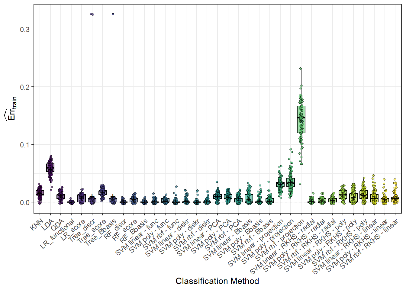

Figure 6.25: Box plots of training errors for 100 simulations separately for each classification method. The black symbols \(+\) denote the means.

Code

# for testing data
SIMULACE$test |> 
  pivot_longer(cols = methods, names_to = 'method', values_to = 'Err') |>
  mutate(method = factor(method, levels = methods, labels = methods, ordered = TRUE)) |> 
  as.data.frame() |>
   filter(method %in% sub_methods) |>
  ggplot(aes(x = method, y = Err, fill = method, colour = method, alpha = method)) +
  geom_jitter(position = position_jitter(height = 0, width = 0.15), alpha = 0.6, size = 0.9, pch = 21,
              colour = "black") +
  geom_boxplot(outlier.colour = "white", outlier.shape = 16, outlier.size = 0, 
               notch = FALSE, colour = 'black') + 
  theme_bw() + 
  labs(x = 'Classification Method',
       y = "$\\widehat{\\textnormal{Err}}_{test}$"
       # y = expression(widehat(Err)[train])
       ) + 
  theme(legend.position = 'none',
        axis.text.x = element_text(angle = 45, hjust = 1)) +
  stat_summary(fun = "mean", geom = "point", shape = 4,
               size = 2, color = "black", alpha = 1) +
  scale_x_discrete(labels = methods_names1) +
  theme(plot.margin = unit(c(0.1, 0.1, 0.7, 0.5), "cm")) +
  coord_cartesian(ylim = c(0, 0.15)) +
  scale_fill_manual(values = box_col1) +
  scale_alpha_manual(values = box_alpha1) +
  geom_hline(yintercept = min(SIMULACE.df$Err.test), 
             linetype = 'dashed', colour = 'grey20', alpha = 0.8)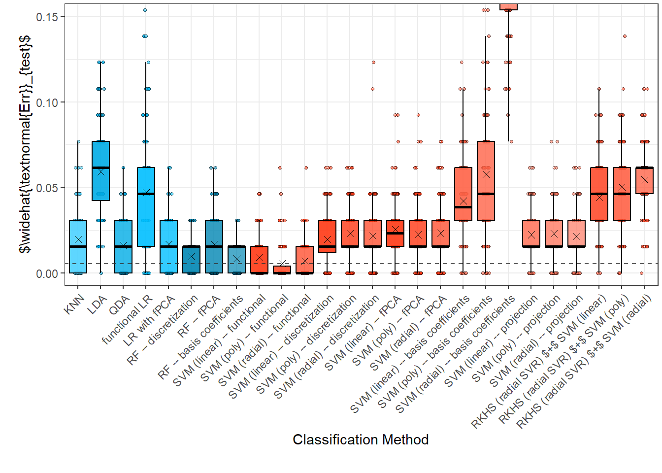

Figure 6.26: Box plots of testing errors for 100 simulations separately for each classification method. The black symbols \(+\) denote the means.

Code

# ggsave("figures/results_tec_der.tex", device = tikz, width = 7, height = 5)
# ggsave("figures/kap7_tecator_box_test_der_subset.tex", device = tikz, width = 6.5, height = 5)

Finally, let’s take a look at which hyperparameter values were the most commonly chosen.

Table 5.16: Medians of hyperparameter values for selected methods where a hyperparameter was determined using cross-validation.

	Median hyperparameter value
KNN_K	4.0
nharm	2.0
LR_func_n_basis	8.0
SVM_d_Linear	6.0
SVM_d_Poly	6.0
SVM_d_Radial	6.0
SVM_RKHS_radial_gamma1	0.5
SVM_RKHS_radial_gamma2	0.3
SVM_RKHS_radial_gamma3	0.3
SVM_RKHS_radial_d1	14.0
SVM_RKHS_radial_d2	12.0
SVM_RKHS_radial_d3	8.0
SVM_RKHS_poly_p1	4.0
SVM_RKHS_poly_p2	4.0
SVM_RKHS_poly_p3	4.0
SVM_RKHS_poly_d1	6.0
SVM_RKHS_poly_d2	5.0
SVM_RKHS_poly_d3	4.0
SVM_RKHS_linear_d1	21.0
SVM_RKHS_linear_d2	21.0
SVM_RKHS_linear_d3	25.0

Code

CV_res <- CV_RESULTS |> 
  pivot_longer(cols = CV_RESULTS |> colnames(), names_to = 'method', values_to = 'hyperparameter') |>
  mutate(method = factor(method, 
                         levels = CV_RESULTS |> colnames(), 
                         labels = CV_RESULTS |> colnames(), ordered = TRUE)) |> 
  as.data.frame() 

CV_res |> 
  filter(method %in% c('KNN_K', 'nharm', 'LR_func_n_basis')) |>
  ggplot(aes(x = hyperparameter, #y = after_stat(density),
             fill = method, colour = method)) + 
  geom_histogram(binwidth = 1, alpha = 0.6) + 
  theme_bw() + 
  facet_grid(~method, scales = 'free') +
  labs(x = 'Hyperparameter values',
       y = 'Absolute count') + 
  theme(legend.position = 'none')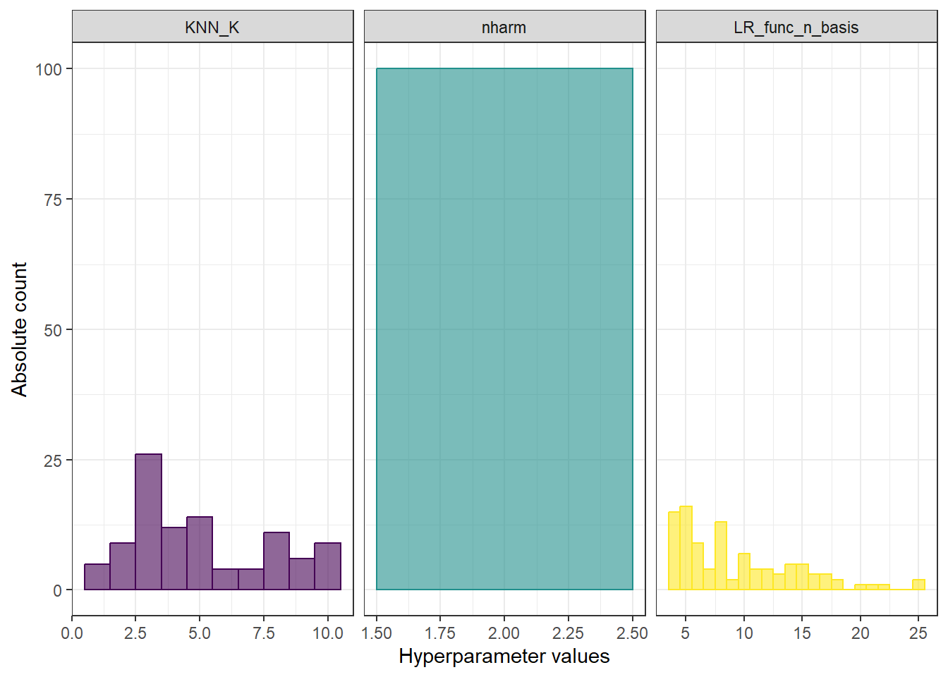

Figure 5.41: Histograms of hyperparameter values for KNN, functional logistic regression, and also a histogram for the number of principal components.

Code

CV_res |> 
  filter(method %in% c('SVM_d_Linear', 'SVM_d_Poly', 'SVM_d_Radial')) |>
  ggplot(aes(x = hyperparameter, #y = after_stat(density),
             fill = method, colour = method)) + 
  geom_histogram(binwidth = 1, alpha = 0.6) + 
  theme_bw() + 
  facet_grid(~method, scales = 'free') +
  labs(x = 'Hyperparameter values',
       y = 'Absolute count') + 
  theme(legend.position = 'none')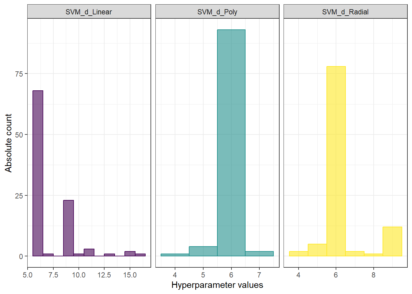

Figure 6.27: Histograms of hyperparameter values for SVM with projection onto B-spline basis.

Code

CV_res |> 
  filter(method %in% c('SVM_RKHS_radial_gamma1', 'SVM_RKHS_radial_gamma2',
                       'SVM_RKHS_radial_gamma3', 'SVM_RKHS_radial_d1', 
                       'SVM_RKHS_radial_d2', 'SVM_RKHS_radial_d3')) |>
  ggplot(aes(x = hyperparameter, #y = after_stat(density),
             fill = method, colour = method)) + 
  geom_histogram(bins = 10, alpha = 0.6) + 
  theme_bw() + 
  facet_wrap(~method, scales = 'free', ncol = 3) +
  labs(x = 'Hyperparameter values',
       y = 'Absolute count') + 
  theme(legend.position = 'none')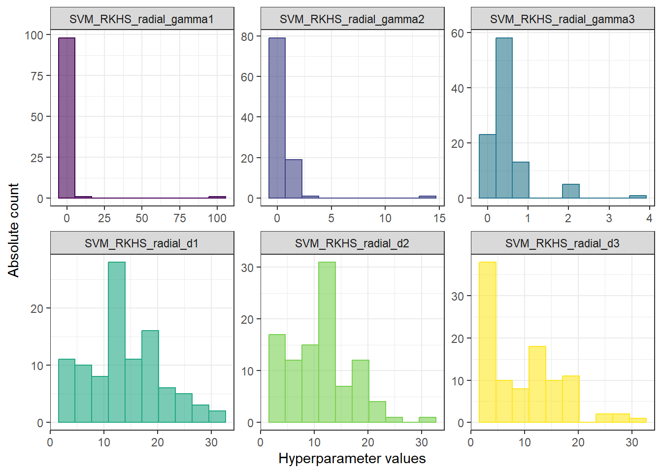

Figure 5.42: Histograms of hyperparameter values for RKHS + SVM with radial kernel.

Code

CV_res |> 
  filter(method %in% c('SVM_RKHS_poly_p1', 'SVM_RKHS_poly_p2',
                       'SVM_RKHS_poly_p3', 'SVM_RKHS_poly_d1',
                       'SVM_RKHS_poly_d2', 'SVM_RKHS_poly_d3')) |>
  ggplot(aes(x = hyperparameter, #y = after_stat(density),
             fill = method, colour = method)) + 
  geom_histogram(binwidth = 1, alpha = 0.6) + 
  theme_bw() + 
  facet_wrap(~method, scales = 'free', ncol = 3) +
  labs(x = 'Hyperparameter values',
       y = 'Absolute count') + 
  theme(legend.position = 'none')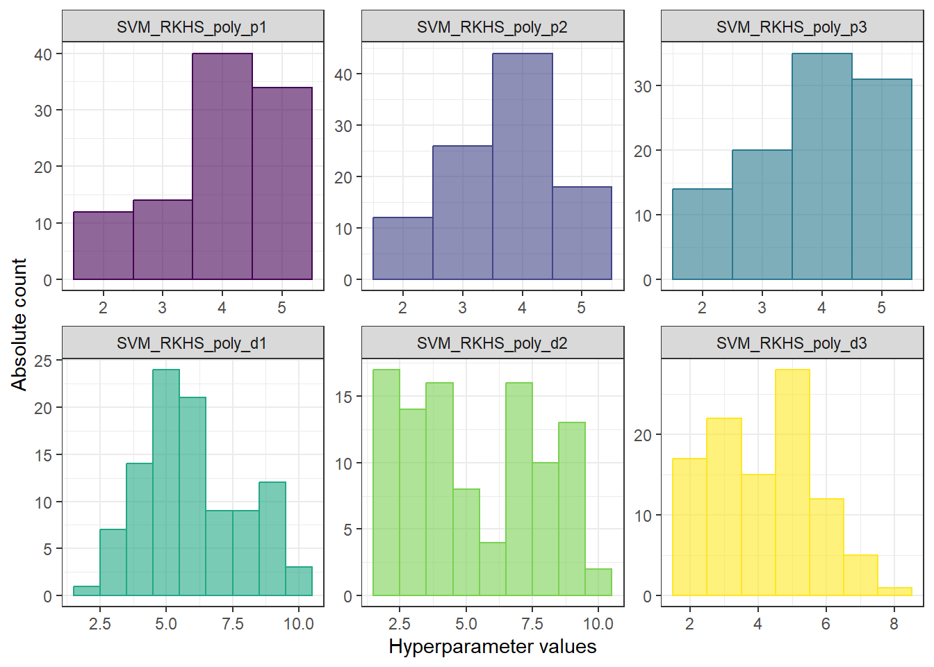

Figure 6.28: Histograms of hyperparameter values for RKHS + SVM with polynomial kernel.

Code

CV_res |> 
  filter(method %in% c('SVM_RKHS_linear_d1',
                       'SVM_RKHS_linear_d2', 'SVM_RKHS_linear_d3')) |>
  ggplot(aes(x = hyperparameter, #y = after_stat(density),
             fill = method, colour = method)) + 
  geom_histogram(binwidth = 5, alpha = 0.6) + 
  theme_bw() + 
  facet_wrap(~method, scales = 'free', ncol = 3) +
  labs(x = 'Hyperparameter values',
       y = 'Absolute count') + 
  theme(legend.position = 'none')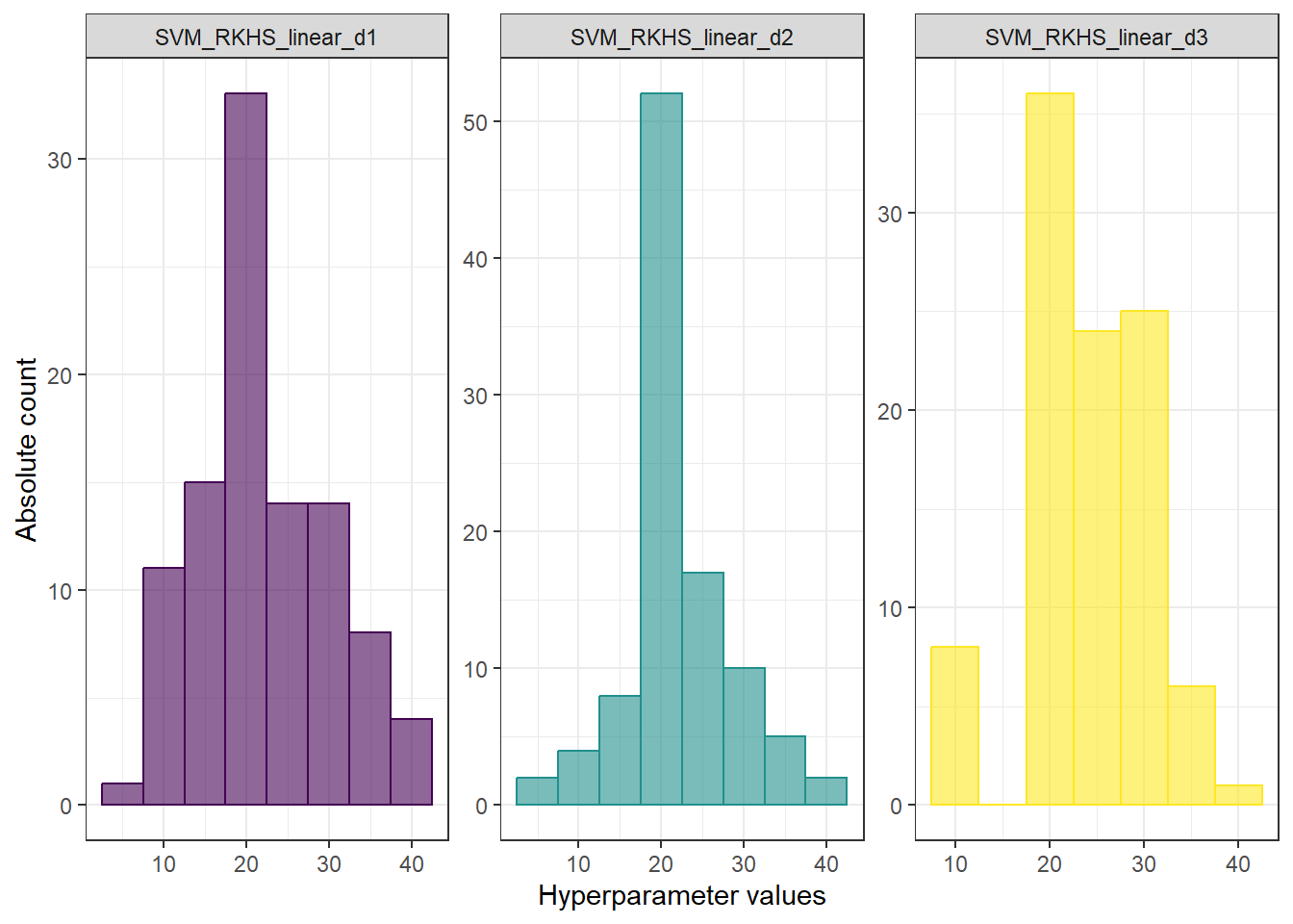

Figure 5.43: Histograms of hyperparameter values for RKHS + SVM with linear kernel.