Chapter 1 Classification of simulated curves

1.1 Simulation of Functional Data

First, we simulate functions that we will subsequently classify. For simplicity, we will consider two classification classes. For the simulation, we will first:

choose appropriate functions,
generate points from a selected interval, which contain, for example, Gaussian noise,
smooth these obtained discrete points into a functional object form using a suitable basis system.

Through this process, we obtain functional objects along with the value of a categorical variable $Y$, which distinguishes membership in the classification class.

Code

library(fda)
library(ggplot2)
library(dplyr)
library(tidyr)
library(ddalpha)
library(polynom)

set.seed(42)

Let us consider two classification classes, $Y \in \{0, 1\}$, with the same number n of generated functions for each class. First, let’s define two functions, each corresponding to one class. We will consider the functions on the interval $I = [0, 6]$.

Now, we will create the functions using interpolation polynomials. First, we define the points through which our curve should pass, and then we fit an interpolation polynomial through them, which we use to generate curves for classification.

Code

# defining points for class 0
x.0 <- c(0.00, 0.65, 0.94, 1.42, 2.26, 2.84, 3.73, 4.50, 5.43, 6.00)
y.0 <- c(0, 0.25, 0.86, 1.49, 1.1, 0.15, -0.11, -0.36, 0.23, 0)

# defining points for class 1
x.1 <- c(0.00, 0.51, 0.91, 1.25, 1.51, 2.14, 2.43, 2.96, 3.70, 4.60,
         5.25, 5.67, 6.00)
y.1 <- c(0.1, 0.4, 0.71, 1.08, 1.47, 1.39, 0.81, 0.05, -0.1, -0.4,
         0.3, 0.37, 0)

Code

dat_points <- data.frame(x = c(x.0, x.1),
                         y = c(y.0, y.1),
                         Class = rep(c('Y = 0', 'Y = 1'), 
                                     c(length(x.0), length(x.1))))

ggplot(dat_points, aes(x = x, y = y, colour = Class)) + 
  geom_point(size=1.5) + 
  theme_bw() + 
  labs(x = expression(x[1]),
       y = expression(x[2]),
       colour = 'Class')

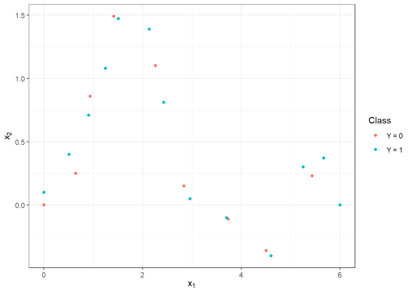
Figure 1.1: Points defining interpolation polynomials for both classification classes.

To compute the interpolation polynomials, we will use the poly.calc() function from the polynom library. Next, we define the functions poly.0() and poly.1(), which will calculate the polynomial values at a given point in the interval. We use the predict() function to create them, where we input the respective polynomial and the point at which we want to evaluate the polynomial.

Code

polynom.0 <- poly.calc(x.0, y.0)
polynom.1 <- poly.calc(x.1, y.1)

Code

poly.0 <- function(x) return(predict(polynom.0, x))
poly.1 <- function(x) return(predict(polynom.1, x))

Code

xx <- seq(min(x.0), max(x.0), length = 501)
yy.0 <- poly.0(xx)
yy.1 <- poly.1(xx)

dat_poly_plot <- data.frame(x = c(xx, xx),
                            y = c(yy.0, yy.1),
                            Class = rep(c('Y = 0', 'Y = 1'), 
                                        c(length(xx), length(xx))))

ggplot(dat_points, aes(x = x, y = y, colour = Class)) + 
  geom_point(size=1.5) + 
  theme_bw() + 
  geom_line(data = dat_poly_plot,
            aes(x = x, y = y, colour = Class),
            linewidth = 0.8) + 
  labs(x = expression(x[1]),
       y = expression(x[2]),
       colour = 'Class')

Figure 1.2: Visualization of two functions on the interval $I = [0, 6]$, from which we generate observations for classes 0 and 1.

Code

funkce_0 <- poly.0
funkce_1 <- poly.1

Now we will create a function to generate random functions with added noise (i.e., points on a predefined grid) from a chosen generating function. The argument t represents the vector of values at which we want to evaluate the given functions, fun denotes the generating function, n is the number of functions, and sigma is the standard deviation $\sigma$ of the normal distribution $\text{N}(\mu, \sigma^2)$, from which we randomly generate Gaussian white noise with $\mu = 0$. To demonstrate the advantage of using methods that work with functional data, we will add a random term to each simulated observation during generation, representing a vertical shift of the entire function (parameter sigma_shift). This shift will be generated from a normal distribution with the parameter $\sigma^2 = 4$.

Code

generate_values <- function(t, fun, n, sigma, sigma_shift = 0) {
  # Arguments:
  # t ... vector of values, where the function will be evaluated
  # fun ... generating function of t 
  # n ... the number of generated functions / objects
  # sigma ... standard deviation of normal distribution to add noise to data
  # sigma_shift ... parameter of normal distribution for generating shift
  
  # Value:
  # X ... matrix of dimension length(t) times n with generated values of one 
  # function in a column 
  
  X <- matrix(rep(t, times = n), ncol = n, nrow = length(t), byrow = FALSE)
  noise <- matrix(rnorm(n * length(t), mean = 0, sd = sigma),
                  ncol = n, nrow = length(t), byrow = FALSE)
  shift <- matrix(rep(rnorm(n, 0, sigma_shift), each = length(t)),
                  ncol = n, nrow = length(t))
  return(fun(X) + noise + shift)
}

Now we can generate the functions. In each of the two classes, we will consider 100 observations, so n = 100.

Code

n <- 100
t <- seq(0, 6, length = 51)

# Y = 0
X0 <- generate_values(t, funkce_0, n, 1, 2)
# Y = 1
X1 <- generate_values(t, funkce_1, n, 1, 2)

We will plot the generated (not yet smoothed) functions in color according to their class (only the first 10 observations from each class for clarity).

Code

n_curves_plot <- 10 

DF0 <- cbind(t, X0[, 1:n_curves_plot]) |> 
  as.data.frame() |> 
  reshape(varying = 2:(n_curves_plot + 1), direction = 'long', sep = '') |> 
  subset(select = -id) |> 
  mutate(
  time = time - 1,
  group = 0
  )

DF1 <- cbind(t, X1[, 1:n_curves_plot]) |> 
  as.data.frame() |> 
  reshape(varying = 2:(n_curves_plot + 1), direction = 'long', sep = '') |> 
  subset(select = -id) |> 
  mutate(
  time = time - 1,
  group = 1
  )

DF <- rbind(DF0, DF1) |>
  mutate(group = factor(group))

DF |> ggplot(aes(x = t, y = V, group = interaction(time, group), 
                 colour = group)) + 
  geom_line(linewidth = 0.5) +
  theme_bw() +
  labs(x = expression(x[1]),
       y = expression(x[2]),
       colour = 'Class') +
  scale_colour_discrete(labels=c('Y = 0', 'Y = 1'))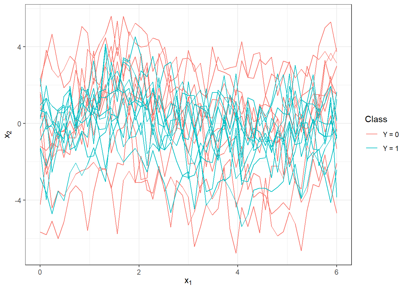

Figure 1.3: The first 10 generated observations from each of the two classification classes. The observed data are not smoothed.

1.2 Smoothing Observed Curves

Now we will convert the observed discrete values (vectors of values) into functional objects that we will work with subsequently. We will again use a B-spline basis for smoothing.

We take the entire vector t as the knots, and since we are considering cubic splines, we choose (the implicit choice in R) norder = 4. We will penalize the second derivative of the functions.

Code

rangeval <- range(t)
breaks <- t
norder <- 4

bbasis <- create.bspline.basis(rangeval = rangeval, 
                               norder = norder, 
                               breaks = breaks)

curv.Lfd <- int2Lfd(2)

We will find a suitable value for the smoothing parameter $\lambda > 0$ using $GCV(\lambda)$, which stands for generalized cross-validation. We will consider the same value of $\lambda$ for both classification groups, as we would not know in advance which value of $\lambda$ to choose for test observations in the case of different selections for each class.

Code

XX <- cbind(X0, X1)

lambda.vect <- 10^seq(from = -4, to = 1, length.out = 50) 
gcv <- rep(NA, length = length(lambda.vect)) 

for(index in 1:length(lambda.vect)) {
  curv.Fdpar <- fdPar(bbasis, curv.Lfd, lambda.vect[index])
  BSmooth <- smooth.basis(t, XX, curv.Fdpar) 
  gcv[index] <- mean(BSmooth$gcv) 
}

GCV <- data.frame(
  lambda = round(log10(lambda.vect), 3),
  GCV = gcv
)

lambda.opt <- lambda.vect[which.min(gcv)]

To better illustrate, we will plot the course of $GCV(\lambda)$.

Code

GCV |> ggplot(aes(x = lambda, y = GCV)) + 
  geom_line(linetype = 'solid', linewidth = 0.6) + 
  geom_point(size = 1.5) + 
  theme_bw() + 
  labs(x = bquote(paste(log[10](lambda), ' ;   ', 
                        lambda[optimal] == .(round(lambda.opt, 4)))),
       y = expression(GCV(lambda))) + 
  geom_point(aes(x = log10(lambda.opt), y = min(gcv)), colour = 'red', size = 2.5)

## Warning in geom_point(aes(x = log10(lambda.opt), y = min(gcv)), colour = "red", : All aesthetics have length 1, but the data has 50 rows.
## ℹ Please consider using `annotate()` or provide this layer with data containing
##   a single row.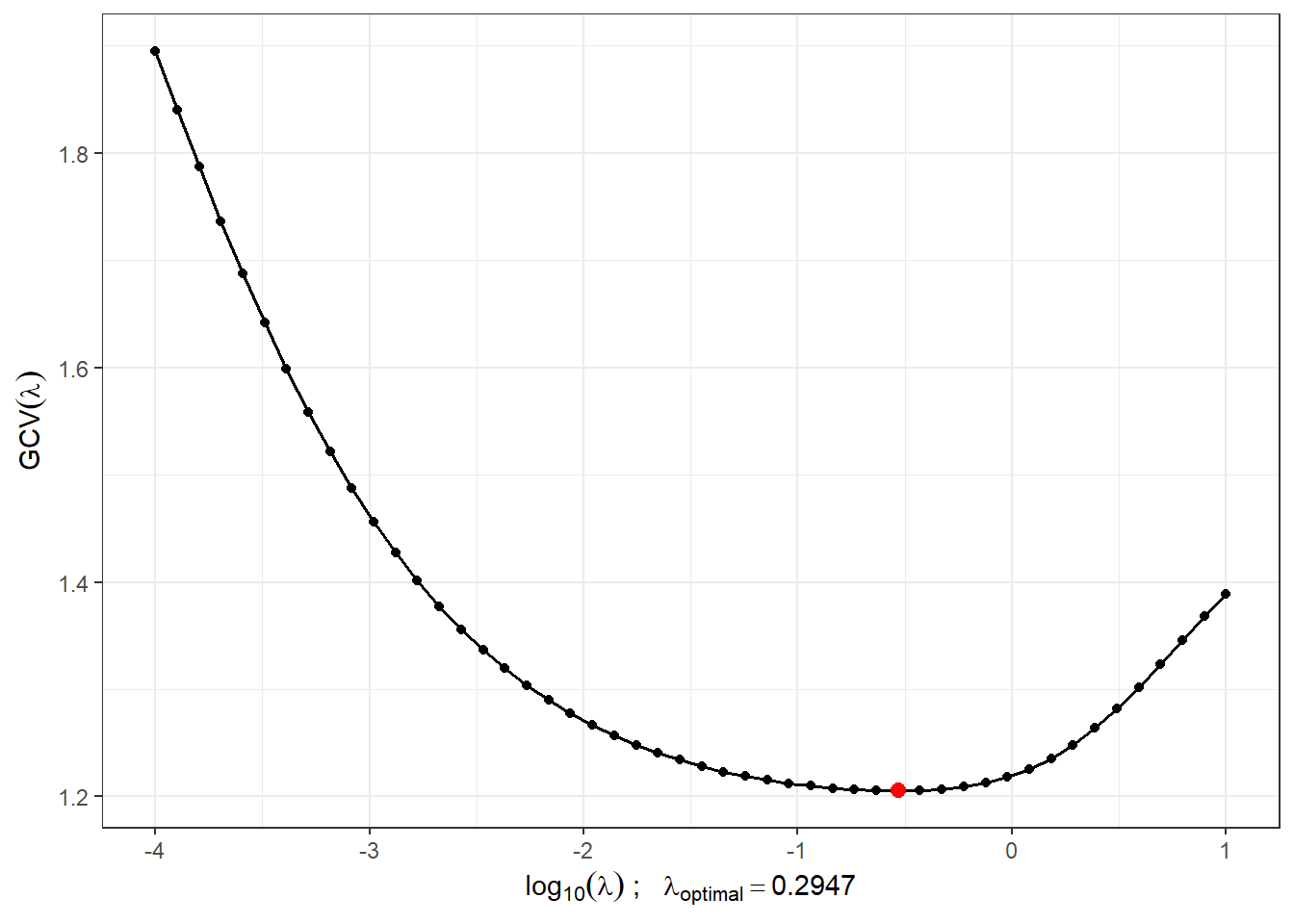

$The course of $GCV(\lambda)$ for the chosen vector $\boldsymbol\lambda$. The values on the $x$-axis are plotted on a logarithmic scale. The optimal value of the smoothing parameter $\lambda_{optimal}$ is indicated in red.$

Figure 1.4: The course of $GCV(\lambda)$ for the chosen vector $\boldsymbol\lambda$. The values on the $x$-axis are plotted on a logarithmic scale. The optimal value of the smoothing parameter $\lambda_{optimal}$ is indicated in red.

With this optimal choice of the smoothing parameter $\lambda$, we will now smooth all functions and again graphically represent the first 10 observed curves from each classification class.

Code

curv.fdPar <- fdPar(bbasis, curv.Lfd, lambda.opt)
BSmooth <- smooth.basis(t, XX, curv.fdPar)
XXfd <- BSmooth$fd

fdobjSmootheval <- eval.fd(fdobj = XXfd, evalarg = t)
DF$Vsmooth <- c(fdobjSmootheval[, c(1 : n_curves_plot, 
                                    (n + 1) : (n + n_curves_plot))])

DF |> ggplot(aes(x = t, y = Vsmooth, group = interaction(time, group), 
                 colour = group)) + 
  geom_line(linewidth = 0.75) +
  theme_bw() +
  labs(x = expression(x[1]),
       y = expression(x[2]),
       colour = 'Class') +
  scale_colour_discrete(labels=c('Y = 0', 'Y = 1'))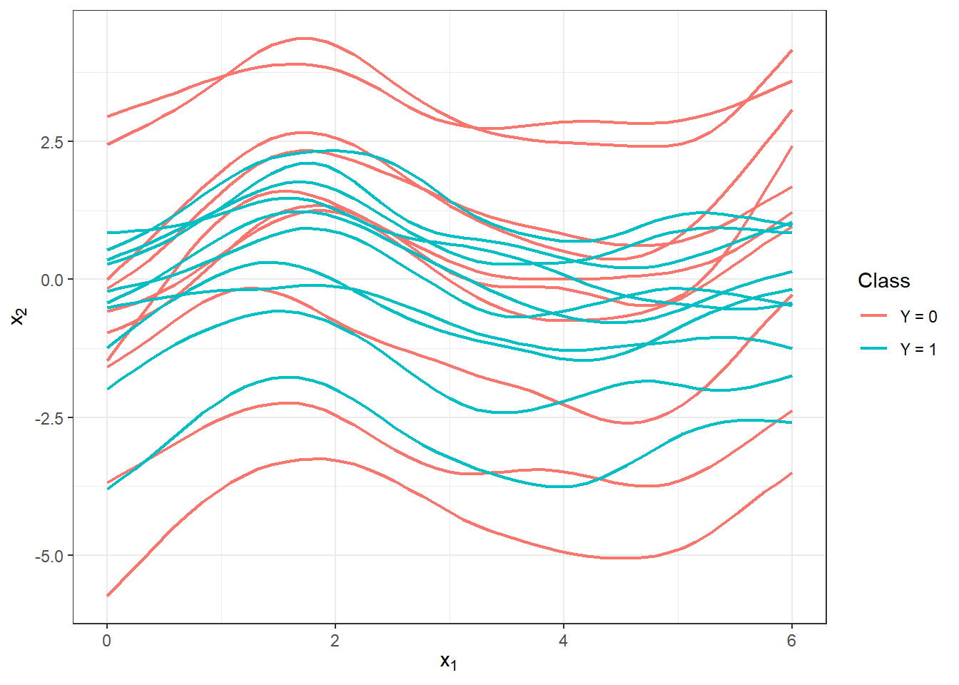

Figure 1.5: The first 10 smoothed curves from each classification class.

Let’s also illustrate all curves, including the average, separately for each class.

Code

abs.labs <- paste("Classification class:", c("$Y = 0$", "$Y = 1$"))
names(abs.labs) <- c('0', '1')

fdobjSmootheval <- eval.fd(fdobj = XXfd, evalarg = t)

DFsmooth <- data.frame(
  t = rep(t, 2 * n),
  time = rep(rep(1:n, each = length(t)), 2),
  Smooth = c(fdobjSmootheval),
  group = factor(rep(c(0, 1), each = n * length(t)))
)

DFmean <- data.frame(
  t = rep(t, 2),
  Mean = c(eval.fd(fdobj = mean.fd(XXfd[1:n]), evalarg = t),
           eval.fd(fdobj = mean.fd(XXfd[(n + 1):(2 * n)]), evalarg = t)),
  group = factor(rep(c(0, 1), each = length(t)))
)

DFsmooth |> ggplot(aes(x = t, y = Smooth, #group = interaction(time, group), 
                 colour = group)) + 
  geom_line(aes(group = time), linewidth = 0.05, alpha = 0.5) +
  theme_bw() +
  labs(x = "$t$",
       y = "$x_i(t)$",
       colour = 'Class') +
  # geom_line(data = DFsmooth |> 
  #             mutate(group = factor(ifelse(group == '0', '1', '0'))) |> 
  #             filter(group == '1'),
  #           aes(x = t, y = Mean, colour = group), 
  #           colour = 'tomato', linewidth = 0.8, linetype = 'solid') + 
  # geom_line(data = DFsmooth |> 
  #             mutate(group = factor(ifelse(group == '0', '1', '0'))) |> 
  #             filter(group == '0'),
  #           aes(x = t, y = Mean, colour = group), 
  #           colour = 'deepskyblue2', linewidth = 0.8, linetype = 'solid') + 
  geom_line(data = DFmean |> 
              mutate(group = factor(ifelse(group == '0', '1', '0'))),
            aes(x = t, y = Mean, colour = group), 
            colour = 'grey2', linewidth = 0.8, linetype = 'dashed') + 
  geom_line(data = DFmean, aes(x = t, y = Mean, colour = group), 
            colour = 'grey2', linewidth = 1.25, linetype = 'solid') + 
  scale_x_continuous(expand = c(0.01, 0.01)) +
  facet_wrap(~group, labeller = labeller(group = abs.labs)) +
  scale_y_continuous(expand = c(0.02, 0.02)) +
  theme(legend.position = 'none') +
  scale_colour_manual(values = c('tomato', 'deepskyblue2'))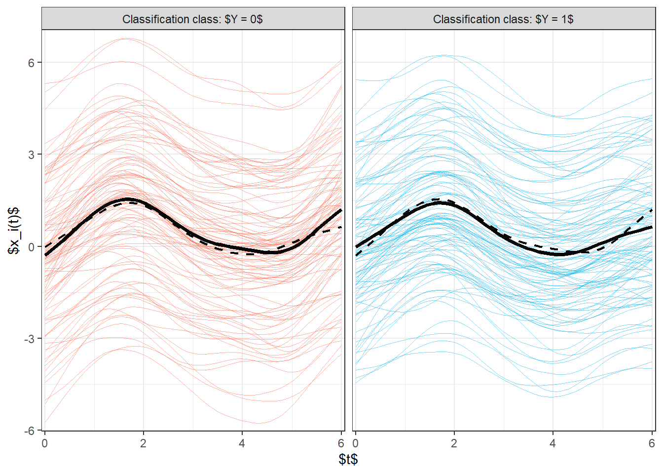

Plot of all smoothed observed curves, distinguished by color according to their classification class. The average for each class is indicated by a black line, and for the second class, it is indicated by a dashed line.

Figure 1.6: Plot of all smoothed observed curves, distinguished by color according to their classification class. The average for each class is indicated by a black line, and for the second class, it is indicated by a dashed line.

Code

# ggsave("figures/kap6_sim_03_curves.tex", device = tikz, width = 8, height = 4)

Now let’s take a look at the comparison of average courses from a detailed perspective.

Code

DFsmooth <- data.frame(
  t = rep(t, 2 * n),
  time = rep(rep(1:n, each = length(t)), 2),
  Smooth = c(fdobjSmootheval),
  Mean = c(rep(apply(fdobjSmootheval[ , 1 : n], 1, mean), n),
            rep(apply(fdobjSmootheval[ , (n + 1) : (2 * n)], 1, mean), n)),
  group = factor(rep(c(0, 1), each = n * length(t)))
)

DFmean <- data.frame(
  t = rep(t, 2),
  Mean = c(apply(fdobjSmootheval[ , 1 : n], 1, mean), 
            apply(fdobjSmootheval[ , (n + 1) : (2 * n)], 1, mean)),
  group = factor(rep(c(0, 1), each = length(t)))
)

DFsmooth |> ggplot(aes(x = t, y = Smooth, group = interaction(time, group), 
                 colour = group)) + 
  geom_line(linewidth = 0.25, alpha = 0.5) +
  theme_bw() +
  labs(x = expression(x[1]),
       y = expression(x[2]),
       colour = 'Class') +
  scale_colour_discrete(labels = c('Y = 0', 'Y = 1')) + 
  geom_line(aes(x = t, y = Mean, colour = group), 
            linewidth = 1.2, linetype = 'solid') + 
  scale_x_continuous(expand = c(0.01, 0.01)) + 
  #ylim(c(-1, 2)) + 
  scale_y_continuous(expand = c(0.01, 0.01), limits = c(-1, 2))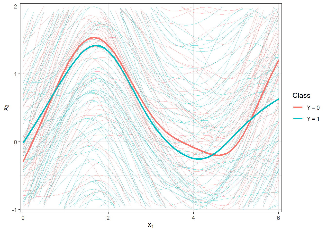

Figure 1.7: Plot of all smoothed observed curves, distinguished by color according to their classification class. The average for each class is indicated by a black line. A closer view.

1.3 Classification of Curves

First, we will load the necessary libraries for classification.

Code

library(caTools) 
library(caret) 
library(fda.usc) 
library(MASS)
library(fdapace)
library(pracma)
library(refund)
library(nnet) 
library(caret)
library(rpart) 
library(rattle) 
library(e1071)
library(randomForest)

To compare the individual classifiers, we will split the set of generated observations into two parts in a ratio of 70:30, designating them as the training and test (validation) sets. The training set will be used for constructing the classifier, while the test set will be used to calculate the classification error and potentially other characteristics of our model. We can then compare the resulting classifiers based on these calculated characteristics in terms of their classification success.

Code

# Splitting into test and training sets
split <- sample.split(XXfd$fdnames$reps, SplitRatio = 0.7)

Y <- rep(c(0, 1), each = n)

X.train <- subset(XXfd, split == TRUE)
X.test <- subset(XXfd, split == FALSE)

Y.train <- subset(Y, split == TRUE)
Y.test <- subset(Y, split == FALSE)

Next, let’s look at the representation of individual groups in the test and training portions of the data.

Code

# Absolute representation
table(Y.train)

## Y.train
##  0  1 
## 71 69

Code

table(Y.test)

## Y.test
##  0  1 
## 29 31

Code

# Relative representation
table(Y.train) / sum(table(Y.train))

## Y.train
##         0         1 
## 0.5071429 0.4928571

Code

table(Y.test) / sum(table(Y.test))

## Y.test
##         0         1 
## 0.4833333 0.5166667

1.3.1 $K$-Nearest Neighbors

Let’s start with the non-parametric classification method, specifically the $K$-nearest neighbors method. First, we will create the necessary objects so that we can work with them using the classif.knn() function from the fda.usc library.

Code

x.train <- fdata(X.train)
y.train <- as.numeric(factor(Y.train))

Now we can define the model and examine its classification success. However, the last question remains: how do we choose the optimal number of neighbors $K$? We could select $K$ as the value that results in the minimum error on the training data. However, this could lead to overfitting, so we will use cross-validation. Given the computational intensity and the size of the dataset, we will choose $k$-fold cross-validation; for example, we will set $k = 10$.

Code

# Model for all training data for K = 1, 2, ..., sqrt(n_train)
neighb.model <- classif.knn(group = y.train, 
                            fdataobj = x.train, 
                            knn = c(1:round(sqrt(length(y.train))))) 

# neighb.model$max.prob # Maximum accuracy
# (K.opt <- neighb.model$h.opt) # Optimal value of K

Let’s perform the previous procedure for the training data, which we will split into $k$ parts and repeat this part of the code $k$ times.

Code

k_cv <- 10 # k-fold CV
neighbours <- c(1:(2 * ceiling(sqrt(length(y.train))))) # Number of neighbors

# Splitting training data into k parts
folds <- createMultiFolds(X.train$fdnames$reps, k = k_cv, time = 1)

# Empty matrix to store individual results
# Columns will have accuracy values for the given part of the training set
# Rows will have values for the given neighbor count K
CV.results <- matrix(NA, nrow = length(neighbours), ncol = k_cv)

for (index in 1:k_cv) {
  # Define the current index set
  fold <- folds[[index]]
    
  x.train.cv <- subset(X.train, c(1:length(X.train$fdnames$reps)) %in% fold) |>
    fdata()
  y.train.cv <- subset(Y.train, c(1:length(X.train$fdnames$reps)) %in% fold) |>
    factor() |> as.numeric()
  
  x.test.cv <- subset(X.train, !c(1:length(X.train$fdnames$reps)) %in% fold) |>
    fdata()
  y.test.cv <- subset(Y.train, !c(1:length(X.train$fdnames$reps)) %in% fold) |>
    factor() |> as.numeric()
  
  # Iterate through each part... repeat k times
  for(neighbour in neighbours) {
    # Model for the specific choice of K
    neighb.model <- classif.knn(group = y.train.cv, 
                              fdataobj = x.train.cv, 
                              knn = neighbour) 
    # Prediction on the validation part
    model.neighb.predict <- predict(neighb.model, 
                                    new.fdataobj = x.test.cv)
    # Accuracy on the validation part
    accuracy <- table(y.test.cv, model.neighb.predict) |> 
      prop.table() |> diag() |> sum()
    
    # Store the accuracy in the position for the given K and fold
    CV.results[neighbour, index] <- accuracy
  }
}

# Calculate average accuracies for each K across folds
CV.results <- apply(CV.results, 1, mean)
K.opt <- which.max(CV.results)
accuracy.opt.cv <- max(CV.results)
# CV.results

We can see that the optimal value of the parameter $K$ is 5 with an error rate calculated using 10-fold CV of 0.3429. For clarity, let’s plot the validation error as a function of the number of neighbors $K$.

Code

CV.results <- data.frame(K = neighbours, CV = CV.results)
CV.results |> ggplot(aes(x = K, y = 1 - CV)) + 
  geom_line(linetype = 'dashed', colour = 'grey') + 
  geom_point(size = 1.5) + 
  geom_point(aes(x = K.opt, y = 1 - accuracy.opt.cv), colour = 'red', size = 2) +
  theme_bw() + 
  labs(x = bquote(paste(K, ' ;   ', 
                        K[optimal] == .(K.opt))),
       y = 'Validation error') + 
  scale_x_continuous(breaks = neighbours)

## Warning in geom_point(aes(x = K.opt, y = 1 - accuracy.opt.cv), colour = "red", : All aesthetics have length 1, but the data has 24 rows.
## ℹ Please consider using `annotate()` or provide this layer with data containing
##   a single row.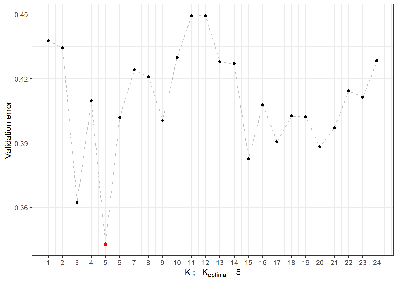

Figure 1.8: Dependence of validation error on the value of $K$, i.e., on the number of neighbors.

Now that we know the optimal value of the parameter $K$, we can construct the final model.

Code

neighb.model <- classif.knn(group = y.train, fdataobj = x.train, knn = K.opt)

# Prediction
model.neighb.predict <- predict(neighb.model, 
                                new.fdataobj = fdata(X.test))

# Accuracy on the test data
accuracy <- table(as.numeric(factor(Y.test)), model.neighb.predict) |>
  prop.table() |>
  diag() |>
  sum()

Thus, we can see that the error rate of the model constructed using the $K$-nearest neighbors method with the optimal choice $K_{optimal}$ equal to 5, which we determined via cross-validation, is 0.3571 on the training data and 0.3833 on the test data.

To compare the different models, we can use both types of errors. For clarity, we will store them in a table.

Code

RESULTS <- data.frame(model = 'KNN', 
                      Err.train = 1 - neighb.model$max.prob,
                      Err.test = 1 - accuracy)

1.3.2 Linear Discriminant Analysis

As the second method for constructing a classifier, we will consider Linear Discriminant Analysis (LDA). Since this method cannot be applied to functional data, we must first discretize it, which we will do using Functional Principal Component Analysis. We will then perform the classification algorithm on the scores of the first $p$ principal components. We will choose the number of components $p$ such that the first $p$ principal components explain at least 90% of the variability in the data.

Let’s first perform Functional Principal Component Analysis and determine the number $p$.

Code

# Principal component analysis
data.PCA <- pca.fd(X.train, nharm = 10) # nharm - maximum number of principal components
nharm <- which(cumsum(data.PCA$varprop) >= 0.9)[1] # determine p
if(nharm == 1) nharm <- 2 # to plot graphs, we need at least 2 principal components

data.PCA <- pca.fd(X.train, nharm = nharm) 
data.PCA.train <- as.data.frame(data.PCA$scores) # scores of the first p principal components
data.PCA.train$Y <- factor(Y.train) # class membership

In this specific case, we took the number of principal components $p = $ 2, which together explain 98.72 % of the variability in the data. The first principal component explains 98.2 % and the second 0.52 % of the variability. We can graphically display the scores of the first two principal components, color-coded according to class membership.

Code

data.PCA.train |> ggplot(aes(x = V1, y = V2, colour = Y)) +
  geom_point(size = 1.5) + 
  labs(x = paste('1st principal component (explained variability', 
                 round(100 * data.PCA$varprop[1], 2), '%)'),
       y = paste('2nd principal component (', 
                 round(100 * data.PCA$varprop[2], 2), '%)'),
       colour = 'Class') +
  scale_colour_discrete(labels = c('Y = 0', 'Y = 1')) +
  theme_bw()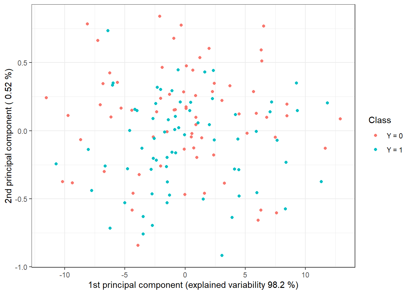

Figure 1.9: Scores of the first two principal components for training data. Points are color-coded according to class membership.

To determine the classification accuracy on the test data, we need to compute the scores for the first 2 principal components for the test data. These scores are calculated using the formula:

\[ \xi_{i, j} = \int \left( X_i(t) - \mu(t)\right) \cdot \rho_j(t)\text dt, \] where $\mu(t)$ is the mean function and $\rho_j(t)$ is the eigenfunction (functional principal component).

Code

# Calculate scores for test functions
scores <- matrix(NA, ncol = nharm, nrow = length(Y.test)) # empty matrix

for(k in 1:dim(scores)[1]) {
  xfd = X.test[k] - data.PCA$meanfd[1] # k-th observation - mean function
  scores[k, ] = inprod(xfd, data.PCA$harmonics) 
  # scalar product of the residual and eigenfunctions rho (functional principal components)
}

data.PCA.test <- as.data.frame(scores)
data.PCA.test$Y <- factor(Y.test)
colnames(data.PCA.test) <- colnames(data.PCA.train)

Now we can construct the classifier on the training data.

Code

# Model
clf.LDA <- lda(Y ~ ., data = data.PCA.train)

# Accuracy on training data
predictions.train <- predict(clf.LDA, newdata = data.PCA.train)
presnost.train <- table(data.PCA.train$Y, predictions.train$class) |>
  prop.table() |> diag() |> sum()
  
# Accuracy on test data
predictions.test <- predict(clf.LDA, newdata = data.PCA.test)
presnost.test <- table(data.PCA.test$Y, predictions.test$class) |>
  prop.table() |> diag() |> sum()

We have calculated the error rate of the classifier on the training data (41.43 %) and on the test data (40 %).

For graphical representation of the method, we can indicate the decision boundary in the scores of the first two principal components. We will calculate this boundary on a dense grid of points and display it using the geom_contour() function.

Code

# Add decision boundary
np <- 1001 # number of grid points
# x-axis ... 1st PC
nd.x <- seq(from = min(data.PCA.train$V1), 
            to = max(data.PCA.train$V1), length.out = np)
# y-axis ... 2nd PC
nd.y <- seq(from = min(data.PCA.train$V2), 
            to = max(data.PCA.train$V2), length.out = np)
# case for 2 PCs ... p = 2
nd <- expand.grid(V1 = nd.x, V2 = nd.y)
# if p = 3
if(dim(data.PCA.train)[2] == 4) {
  nd <- expand.grid(V1 = nd.x, V2 = nd.y, V3 = data.PCA.train$V3[1])}
# if p = 4
if(dim(data.PCA.train)[2] == 5) {
  nd <- expand.grid(V1 = nd.x, V2 = nd.y, V3 = data.PCA.train$V3[1],
                    V4 = data.PCA.train$V4[1])}
# if p = 5
if(dim(data.PCA.train)[2] == 6) {
  nd <- expand.grid(V1 = nd.x, V2 = nd.y, V3 = data.PCA.train$V3[1],
                    V4 = data.PCA.train$V4[1], V5 = data.PCA.train$V5[1])}

# Add Y = 0, 1
nd <- nd |> mutate(prd = as.numeric(predict(clf.LDA, newdata = nd)$class))

data.PCA.train |> ggplot(aes(x = V1, y = V2, colour = Y)) +
  geom_point(size = 1.5) + 
  labs(x = paste('1st principal component (explained variability', 
                 round(100 * data.PCA$varprop[1], 2), '%)'),
       y = paste('2nd principal component (', 
                 round(100 * data.PCA$varprop[2], 2), '%)'),
       colour = 'Class') +
  scale_colour_discrete(labels = c('Y = 0', 'Y = 1')) +
  theme_bw() +
  geom_contour(data = nd, aes(x = V1, y = V2, z = prd), colour = 'black')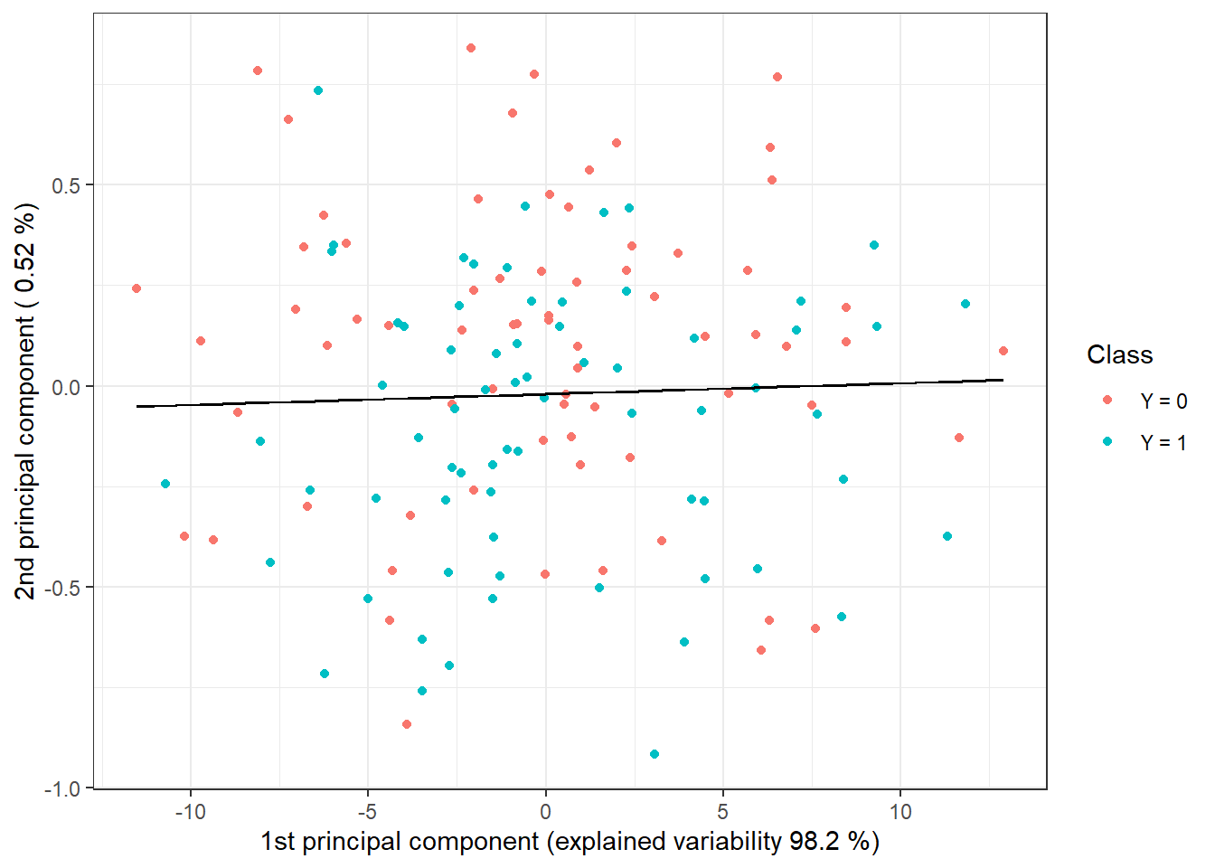

Figure 1.10: Scores of the first two principal components, color-coded according to class membership. The decision boundary (line in the plane of the first two principal components) between the classes constructed using LDA is marked in black.

We see that the decision boundary is a line, a linear function in 2D space, which we expected from LDA. Finally, we will add the error rates to the summary table.

Code

Res <- data.frame(model = 'LDA', 
                  Err.train = 1 - presnost.train,
                  Err.test = 1 - presnost.test)

RESULTS <- rbind(RESULTS, Res)

1.3.3 Quadratic Discriminant Analysis

Next, let’s construct a classifier using Quadratic Discriminant Analysis (QDA). This is an analogous case to LDA, with the difference that we now allow a different covariance matrix for the normal distribution from which the respective scores originate for each of the classes. This relaxed assumption of equal covariance matrices leads to a quadratic boundary between the classes.

In R, we perform QDA analogously to LDA in the previous section, meaning we would again calculate scores for the training and test functions using functional principal component analysis, construct the classifier based on the scores of the first $p$ principal components, and use it to predict the class membership of the test curves $Y^* \in \{0, 1\}$.

We do not need to perform functional PCA; we will use the results from the LDA section.

We can now proceed directly to constructing the classifier, which we will do using the qda() function. We will then calculate the accuracy of the classifier on the test and training data.

Code

# model
clf.QDA <- qda(Y ~ ., data = data.PCA.train)

# accuracy on training data
predictions.train <- predict(clf.QDA, newdata = data.PCA.train)
presnost.train <- table(data.PCA.train$Y, predictions.train$class) |>
  prop.table() |> diag() |> sum()
  
# accuracy on test data
predictions.test <- predict(clf.QDA, newdata = data.PCA.test)
presnost.test <- table(data.PCA.test$Y, predictions.test$class) |>
  prop.table() |> diag() |> sum()

Thus, we have calculated the error rate of the classifier on the training (35.71 %) and test data (40 %).

For a graphical representation of the method, we can mark the decision boundary in the graph of the scores of the first two principal components. We will calculate this boundary on a dense grid of points and display it using the geom_contour() function, just as we did in the case of LDA.

Code

nd <- nd |> mutate(prd = as.numeric(predict(clf.QDA, newdata = nd)$class))

data.PCA.train |> ggplot(aes(x = V1, y = V2, colour = Y)) +
  geom_point(size = 1.5) + 
  labs(x = paste('1st principal component (explained variability', 
                 round(100 * data.PCA$varprop[1], 2), '%)'),
       y = paste('2nd principal component (', 
                 round(100 * data.PCA$varprop[2], 2), '%)'),
       colour = 'Class') +
  scale_colour_discrete(labels = c('Y = 0', 'Y = 1')) +
  theme_bw() +
  geom_contour(data = nd, aes(x = V1, y = V2, z = prd), colour = 'black')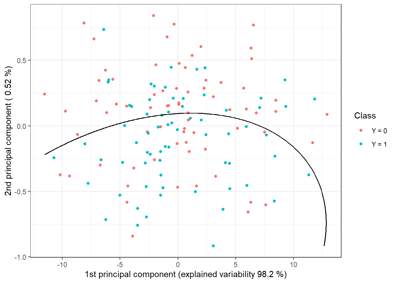

Scores of the first two principal components, colored according to class membership. The decision boundary (a parabola in the plane of the first two principal components) between the classes constructed using QDA is indicated in black.

Figure 1.11: Scores of the first two principal components, colored according to class membership. The decision boundary (a parabola in the plane of the first two principal components) between the classes constructed using QDA is indicated in black.

Note that the decision boundary between the classification classes is now a parabola.

Finally, we will add the error rates to the summary table.

Code

Res <- data.frame(model = 'QDA', 
                  Err.train = 1 - presnost.train,
                  Err.test = 1 - presnost.test)

RESULTS <- rbind(RESULTS, Res)

1.3.4 Logistic Regression

Logistic regression can be conducted in two ways. One way is to use the functional equivalent of classical logistic regression, and the other is the classical multivariate logistic regression applied to scores of the first $p$ principal components.

1.3.4.1 Functional Logistic Regression

Similarly to the case of finite-dimensional input data, we consider the logistic model in the form:

\[ g\left(\mathbb E [Y|X = x]\right) = \eta (x) = g(\pi(x)) = \alpha + \int \beta(t)\cdot x(t) \text d t, \] where $\eta(x)$ is a linear predictor taking values from the interval $(-\infty, \infty)$, $g(\cdot)$ is the link function, which in the case of logistic regression is the logit function $g: (0,1) \rightarrow \mathbb R,\ g(p) = \ln\frac{p}{1-p}$, and $\pi(x)$ is the conditional probability

\[ \pi(x) = \text{Pr}(Y = 1 | X = x) = g^{-1}(\eta(x)) = \frac{\text e^{\alpha + \int \beta(t)\cdot x(t) \text d t}}{1 + \text e^{\alpha + \int \beta(t)\cdot x(t) \text d t}}, \]

where $\alpha$ is a constant and $\beta(t) \in L^2[a, b]$ is the parametric function. Our goal is to estimate this parametric function.

For functional logistic regression, we use the function fregre.glm() from the fda.usc package. First, we create suitable objects for constructing the classifier.

Code

# create suitable objects
x.train <- fdata(X.train)
y.train <- as.numeric(Y.train)

# points where the functions are evaluated
tt <- x.train[["argvals"]]

dataf <- as.data.frame(y.train) 
colnames(dataf) <- "Y"
# B-spline basis 
basis1 <- X.train$basis

To estimate the parametric function $\beta(t)$, we need to express it in some basis representation, in our case a B-spline basis. However, we need to find a suitable number of basis functions for this. This could be determined based on the error on the training data, but such data would favor selecting a large number of bases, leading to model overfitting.

Let’s illustrate this with the following example. For each number of bases $n_{basis} \in \{4, 5, \dots, 50\}$, we train the model on the training data, determine the error on them, and also calculate the error on the test data. Let us recall that we cannot use the same data for selecting the optimal number of bases as for estimating the test error, as this would lead to an underestimated error.

Code

n.basis.max <- 50
n.basis <- 4:n.basis.max
pred.baz <- matrix(NA, nrow = length(n.basis), ncol = 2, 
                   dimnames = list(n.basis, c('Err.train', 'Err.test')))

for (i in n.basis) {
  # basis for betas
  basis2 <- create.bspline.basis(rangeval = range(tt), nbasis = i)
  # relationship
  f <- Y ~ x
  # basis for x and betas
  basis.x <- list("x" = basis1) # smoothed data
  basis.b <- list("x" = basis2)
  # input data for the model
  ldata <- list("df" = dataf, "x" = x.train)
  # binomial model ... logistic regression model
  model.glm <- fregre.glm(f, family = binomial(), data = ldata,
                          basis.x = basis.x, basis.b = basis.b)
  
  # accuracy on training data
  predictions.train <- predict(model.glm, newx = ldata)
  predictions.train <- data.frame(Y.pred = ifelse(predictions.train < 1/2, 0, 1))
  presnost.train <- table(Y.train, predictions.train$Y.pred) |>
    prop.table() |> diag() |> sum()
    
  # accuracy on test data
  newldata = list("df" = as.data.frame(Y.test), "x" = fdata(X.test))
  predictions.test <- predict(model.glm, newx = newldata)
  predictions.test <- data.frame(Y.pred = ifelse(predictions.test < 1/2, 0, 1))
  presnost.test <- table(Y.test, predictions.test$Y.pred) |>
    prop.table() |> diag() |> sum()
  
  # insert into matrix
  pred.baz[as.character(i), ] <- 1 - c(presnost.train, presnost.test)
} 

pred.baz <- as.data.frame(pred.baz)
pred.baz$n.basis <- n.basis

Let’s plot the trend of both types of errors in a graph depending on the number of basis functions.

Code

n.basis.beta.opt <- pred.baz$n.basis[which.min(pred.baz$Err.test)]

pred.baz |> ggplot(aes(x = n.basis, y = Err.test)) + 
  geom_line(linetype = 'dashed', colour = 'black') + 
  geom_line(aes(x = n.basis, y = Err.train), colour = 'deepskyblue3', 
            linetype = 'dashed', linewidth = 0.5) + 
  geom_point(size = 1.5) + 
  geom_point(aes(x = n.basis, y = Err.train), colour = 'deepskyblue3', 
             size = 1.5) + 
  geom_point(aes(x = n.basis.beta.opt, y = min(pred.baz$Err.test)),
             colour = 'red', size = 2) +
  theme_bw() + 
  labs(x = bquote(paste(n[basis], ' ;   ', 
                        n[optimal] == .(n.basis.beta.opt))),
        y = 'Error rate')

## Warning: Use of `pred.baz$Err.test` is discouraged.
## ℹ Use `Err.test` instead.

## Warning in geom_point(aes(x = n.basis.beta.opt, y = min(pred.baz$Err.test)), : All aesthetics have length 1, but the data has 47 rows.
## ℹ Please consider using `annotate()` or provide this layer with data containing
##   a single row.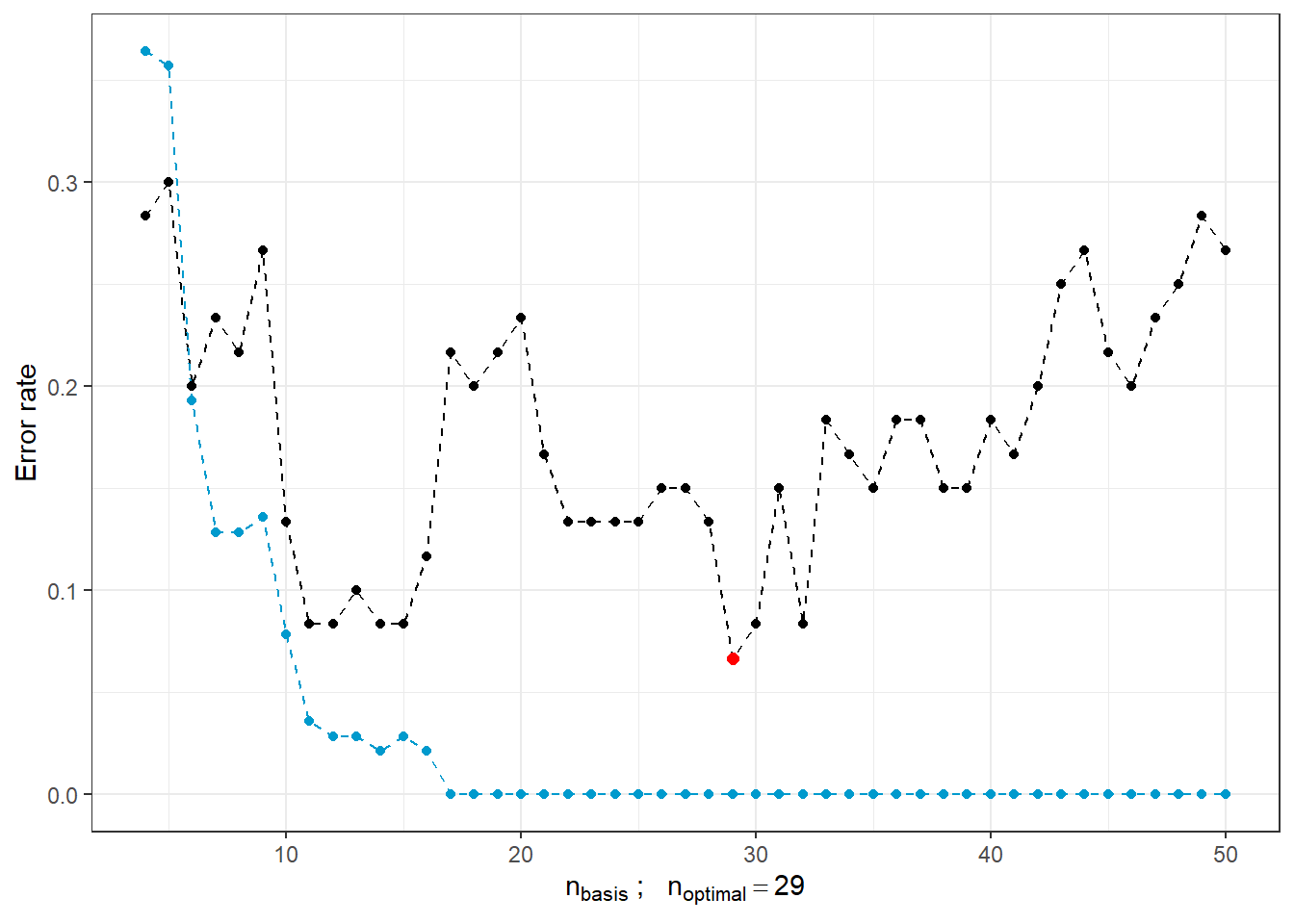

$Dependency of test and training error on the number of basis functions for $\beta$. The optimal number $n_{optimal}$ selected as the minimum test error is marked with a red point, the test error is drawn in black, and the training error is shown with a blue dashed line.$

Figure 1.12: Dependency of test and training error on the number of basis functions for $\beta$. The optimal number $n_{optimal}$ selected as the minimum test error is marked with a red point, the test error is drawn in black, and the training error is shown with a blue dashed line.

We see that as the number of bases for $\beta(t)$ increases, the training error (blue line) tends to decrease, and thus we would select large values of $n_{basis}$ based on it. However, the optimal choice based on the test error is $n$ equal to 29, which is significantly smaller than 50. On the other hand, as $n$ increases, the test error rises, indicating model overfitting.

For these reasons, we use 10-fold cross-validation to determine the optimal number of basis functions for $\beta(t)$. We consider a maximum number of 35 basis functions, as we saw above that beyond this value, the model starts overfitting.

Code

### 10-fold cross-validation
n.basis.max <- 35
n.basis <- 4:n.basis.max
k_cv <- 10 # k-fold CV
# split training data into k parts
folds <- createMultiFolds(X.train$fdnames$reps, k = k_cv, time = 1)
## elements that do not change during the loop
# points where functions are evaluated
tt <- x.train[["argvals"]]
rangeval <- range(tt)
# B-spline basis 
basis1 <- X.train$basis
# relationship
f <- Y ~ x
# basis for x
basis.x <- list("x" = basis1)
# empty matrix to store individual results
# columns contain accuracy values for a given part of the training set
# rows contain values for a given number of bases
CV.results <- matrix(NA, nrow = length(n.basis), ncol = k_cv, 
                     dimnames = list(n.basis, 1:k_cv))

We prepared everything necessary to calculate the error rate for each of the ten subsets of the training set. We then determine the mean error and select the optimal $n$ as the argument of the minimum validation error.

Code

for (index in 1:k_cv) {
  # Define the current index set
  fold <- folds[[index]]
    
  x.train.cv <- subset(X.train, c(1:length(X.train$fdnames$reps)) %in% fold) |>
    fdata()
  y.train.cv <- subset(Y.train, c(1:length(X.train$fdnames$reps)) %in% fold) |>
    as.numeric()
  
  x.test.cv <- subset(X.train, !c(1:length(X.train$fdnames$reps)) %in% fold) |>
    fdata()
  y.test.cv <- subset(Y.train, !c(1:length(X.train$fdnames$reps)) %in% fold) |>
    as.numeric()
  
  dataf <- as.data.frame(y.train.cv) 
  colnames(dataf) <- "Y"
  
  for (i in n.basis) {
    # Basis for betas
    basis2 <- create.bspline.basis(rangeval = rangeval, nbasis = i)
    
    basis.b <- list("x" = basis2)
    # Input data for the model
    ldata <- list("df" = dataf, "x" = x.train.cv)
    # Binomial model... logistic regression model
    model.glm <- fregre.glm(f, family = binomial(), data = ldata,
                            basis.x = basis.x, basis.b = basis.b)
    
    # Accuracy on the validation set
    newldata = list("df" = as.data.frame(y.test.cv), "x" = x.test.cv)
    predictions.valid <- predict(model.glm, newx = newldata)
    predictions.valid <- data.frame(Y.pred = ifelse(predictions.valid < 1/2, 0, 1))
    presnost.valid <- table(y.test.cv, predictions.valid$Y.pred) |>
      prop.table() |> diag() |> sum()
    
    # Insert into the matrix
    CV.results[as.character(i), as.character(index)] <- presnost.valid
  } 
}

# Calculate the average accuracy for each n across folds
CV.results <- apply(CV.results, 1, mean)
n.basis.opt <- n.basis[which.max(CV.results)]
presnost.opt.cv <- max(CV.results)

Next, let’s plot the validation error rate, highlighting the optimal value $n_{optimal}$ equal to 11 with validation error 0.072.

Code

CV.results <- data.frame(n.basis = n.basis, CV = CV.results)
CV.results |> ggplot(aes(x = n.basis, y = 1 - CV)) + 
  geom_line(linetype = 'dashed', colour = 'grey') + 
  geom_point(size = 1.5) + 
  geom_point(aes(x = n.basis.opt, y = 1 - presnost.opt.cv), colour = 'red', size = 2) +
  theme_bw() + 
  labs(x = bquote(paste(n[basis], ' ;   ', 
                        n[optimal] == .(n.basis.opt))),
       y = 'Validation Error Rate') + 
  scale_x_continuous(breaks = n.basis) + 
  theme(panel.grid.minor = element_blank())

## Warning in geom_point(aes(x = n.basis.opt, y = 1 - presnost.opt.cv), colour = "red", : All aesthetics have length 1, but the data has 32 rows.
## ℹ Please consider using `annotate()` or provide this layer with data containing
##   a single row.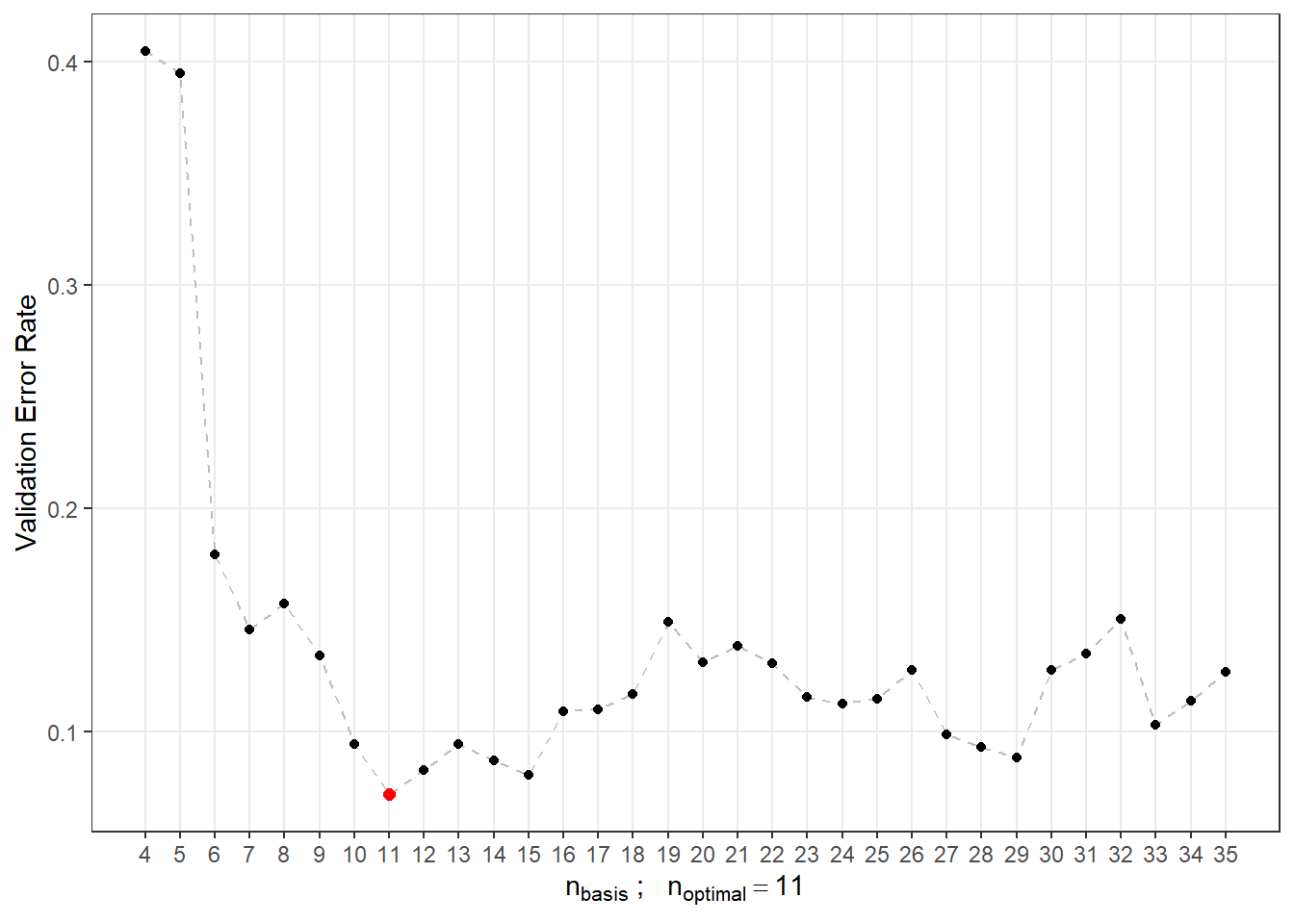

$Relationship of validation error rate with $n_{basis}$, i.e., the number of bases.$

Figure 1.13: Relationship of validation error rate with $n_{basis}$, i.e., the number of bases.

Now we can define the final model using functional logistic regression, choosing a B-spline basis for $\beta(t)$ with 11 bases.

Code

# Optimal model
basis2 <- create.bspline.basis(rangeval = range(tt), nbasis = n.basis.opt)
f <- Y ~ x
# Bases for x and betas
basis.x <- list("x" = basis1) 
basis.b <- list("x" = basis2)
# Input data for the model
dataf <- as.data.frame(y.train) 
colnames(dataf) <- "Y"
ldata <- list("df" = dataf, "x" = x.train)
# Binomial model... logistic regression model
model.glm <- fregre.glm(f, family = binomial(), data = ldata,
                        basis.x = basis.x, basis.b = basis.b)

# Training accuracy
predictions.train <- predict(model.glm, newx = ldata)
predictions.train <- data.frame(Y.pred = ifelse(predictions.train < 1/2, 0, 1))
presnost.train <- table(Y.train, predictions.train$Y.pred) |>
  prop.table() |> diag() |> sum()
  
# Test accuracy
newldata = list("df" = as.data.frame(Y.test), "x" = fdata(X.test))
predictions.test <- predict(model.glm, newx = newldata)
predictions.test <- data.frame(Y.pred = ifelse(predictions.test < 1/2, 0, 1))
presnost.test <- table(Y.test, predictions.test$Y.pred) |>
  prop.table() |> diag() |> sum()

We calculated the training error (equal to 3.57 %) and test error (equal to 8.33 %). For better illustration, we can plot the estimated probabilities of class $Y = 1$ for the training data in relation to the values of the linear predictor.

Code

data.frame(
  linear.predictor = model.glm$linear.predictors,
  response = model.glm$fitted.values,
  Y = factor(y.train)
) |> ggplot(aes(x = linear.predictor, y = response, colour = Y)) + 
  geom_point(size = 1.5) + 
  scale_colour_discrete(labels = c('Y = 0', 'Y = 1')) +
  geom_abline(aes(slope = 0, intercept = 0.5), linetype = 'dashed') + 
  theme_bw() + 
  labs(x = 'Linear Predictor',
       y = 'Estimated Probabilities Pr(Y = 1|X = x)',
       colour = 'Class')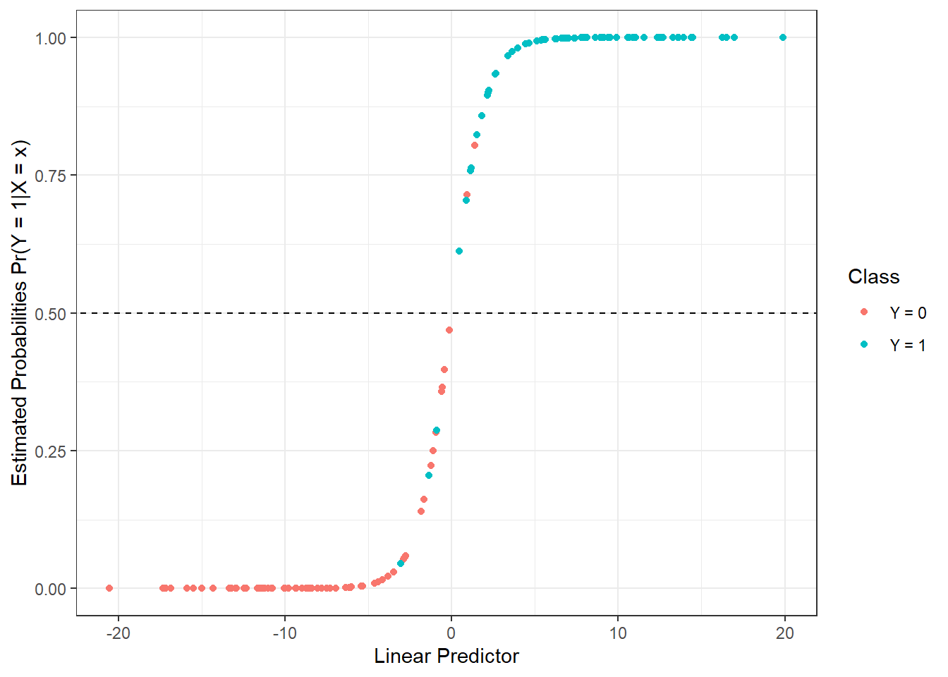

Figure 1.14: Relationship of estimated probabilities with values of the linear predictor. Colors differentiate points by class membership.

For further information, we can also visualize the estimated parametric function $\beta(t)$.

Code

t.seq <- seq(0, 6, length = 1001)
beta.seq <- eval.fd(evalarg = t.seq, fdobj = model.glm$beta.l$x)

data.frame(t = t.seq, beta = beta.seq) |> 
  ggplot(aes(t, beta)) + 
  geom_abline(aes(slope = 0, intercept = 0), linetype = 'dashed', 
              linewidth = 0.5, colour = 'grey') +
  geom_line() + 
  theme_bw() +
  labs(x = expression(x[1]),
       y = expression(widehat(beta)(t))) + 
  theme(panel.grid.major = element_blank(),
        panel.grid.minor = element_blank())

$Plot of the estimated parametric function $\beta(t), t \in [0, 6]$.$

Figure 1.15: Plot of the estimated parametric function $\beta(t), t \in [0, 6]$.

We observe that the values of $\hat\beta(t)$ hover around zero for times $t$ in the middle and beginning of the interval $[0, 6]$, while the values increase for later times. This suggests a distinction between functions of different classes at the beginning and end of the interval, with high similarity in the middle.

Finally, we add the results to the summary table.

Code

Res <- data.frame(model = 'LR functional', 
                  Err.train = 1 - presnost.train,
                  Err.test = 1 - presnost.test)

RESULTS <- rbind(RESULTS, Res)

1.3.4.2 Logistic Regression with Principal Component Analysis

To construct this classifier, we need to perform functional principal component analysis, determine an appropriate number of components, and calculate the score values for the test data. We already performed this in the linear discriminant analysis section, so we will use those results in the following section.

We can now construct the logistic regression model directly using the function glm(, family = binomial).

Code

# model
clf.LR <- glm(Y ~  ., data = data.PCA.train, family = binomial)

# accuracy on training data
predictions.train <- predict(clf.LR, newdata = data.PCA.train, type = 'response')
predictions.train <- ifelse(predictions.train > 0.5, 1, 0)
accuracy.train <- table(data.PCA.train$Y, predictions.train) |>
  prop.table() |> diag() |> sum()
  
# accuracy on test data
predictions.test <- predict(clf.LR, newdata = data.PCA.test, type = 'response')
predictions.test <- ifelse(predictions.test > 0.5, 1, 0)
accuracy.test <- table(data.PCA.test$Y, predictions.test) |>
  prop.table() |> diag() |> sum()

Thus, we calculated the classifier error rate on the training data (40.71 %) and on the test data (40 %).

To illustrate the method graphically, we can plot the decision boundary on a graph of the scores of the first two principal components. This boundary will be calculated on a dense grid of points and displayed using the geom_contour() function, just as in the cases of LDA and QDA.

Code

nd <- nd |> mutate(prd = as.numeric(predict(clf.LR, newdata = nd,
                                            type = 'response')))
nd$prd <- ifelse(nd$prd > 0.5, 1, 0)

data.PCA.train |> ggplot(aes(x = V1, y = V2, colour = Y)) +
  geom_point(size = 1.5) + 
  labs(x = paste('1st Principal Component (explained variability', 
                 round(100 * data.PCA$varprop[1], 2), '%)'),
       y = paste('2nd Principal Component (', 
                 round(100 * data.PCA$varprop[2], 2), '%)'),
       colour = 'Class') +
  scale_colour_discrete(labels = c('Y = 0', 'Y = 1')) +
  theme_bw() +
  geom_contour(data = nd, aes(x = V1, y = V2, z = prd), colour = 'black')

Figure 1.16: Scores of the first two principal components, color-coded by classification class membership. The separating boundary (line in the plane of the first two principal components) between classes, constructed using logistic regression, is shown in black.

Note that the separating boundary between the classification classes is now a line, as in the case of LDA.

Finally, we add the error rates to a summary table.

Code

Res <- data.frame(model = 'LR score', 
                  Err.train = 1 - accuracy.train,
                  Err.test = 1 - accuracy.test)

RESULTS <- rbind(RESULTS, Res)

1.3.5 Decision Trees

In this section, we will look at a very different approach to constructing a classifier compared to methods like LDA or logistic regression. Decision trees are a popular tool for classification; however, as with some previous methods, they are not directly designed for functional data. There are ways, though, to transform functional objects into multivariate form and then apply the decision tree algorithm. We can consider the following approaches:

using the algorithm on basis coefficients,
using principal component scores,
using interval discretization and evaluating the function only on a finite grid of points.

We will first focus on interval discretization and then compare the results with the remaining two approaches for constructing the decision tree.

1.3.5.1 Interval Discretization

First, we need to define points from the interval $I = [0, 6]$ at which we will evaluate the functions. Then, we create an object in which the rows represent individual (discretized) functions, and the columns represent time points. Finally, we add a column $Y$ with the classification class information and repeat the same steps for the test data.

Code

# sequence of points at which the function is evaluated
t.seq <- seq(0, 6, length = 101)
   
grid.data <- eval.fd(fdobj = X.train, evalarg = t.seq)
grid.data <- as.data.frame(t(grid.data)) # transpose for functions in rows
grid.data$Y <- Y.train |> factor()

grid.data.test <- eval.fd(fdobj = X.test, evalarg = t.seq)
grid.data.test <- as.data.frame(t(grid.data.test))
grid.data.test$Y <- Y.test |> factor()

Now we can construct a decision tree where all time points from the t.seq vector serve as predictors. This classifier is not susceptible to multicollinearity, so we don’t need to consider it. Accuracy will be used as the metric.

Code

# model construction
clf.tree <- train(Y ~ ., data = grid.data, 
                 method = "rpart", 
                 trControl = trainControl(method = "CV", number = 10),
                 metric = "Accuracy")

# accuracy on training data
predictions.train <- predict(clf.tree, newdata = grid.data)
accuracy.train <- table(Y.train, predictions.train) |>
  prop.table() |> diag() |> sum()
  
# accuracy on test data
predictions.test <- predict(clf.tree, newdata = grid.data.test)
accuracy.test <- table(Y.test, predictions.test) |>
  prop.table() |> diag() |> sum()

The classifier error rate on the test data is 46.67 % and on the training data 33.57 %.

We can visualize the decision tree using the fancyRpartPlot() function. We set the node colors to reflect the previous color coding. This is an unpruned tree.

Code

colnames(grid.data) <- c(paste0('time:', t.seq), 'Y')
fancyRpartPlot(rpart(Y ~ ., data = grid.data, method = "class"),
               sub = '', palettes = c('Reds', 'Blues'))

Graphic representation of the unpruned decision tree. Nodes belonging to classification class 1 are shown in blue shades, and those for class 0 are in red shades.

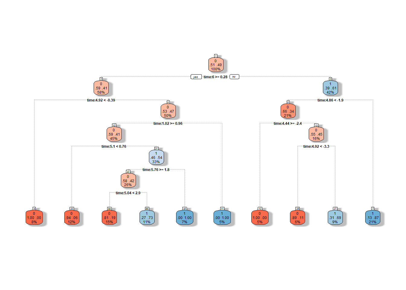
Figure 1.17: Graphic representation of the unpruned decision tree. Nodes belonging to classification class 1 are shown in blue shades, and those for class 0 are in red shades.

We can also plot the final pruned decision tree.

Code

rpart.plot::rpart.plot(clf.tree$finalModel, # final model ... pruned tree
                       extra = 104, # displaying desired information
                       box.palette = c('Reds', 'Blues'),
                       branch.lty = 3, # dotted branch lines
                       shadow.col = 0, # shadows under the node boxes
                       nn = FALSE, 
                       under = FALSE, 
                       digits = 2)

Figure 1.18: Final pruned decision tree.

Finally, we again add the training and test error rates to the summary table.

Code

Res <- data.frame(model = 'Tree - discret.', 
                  Err.train = 1 - accuracy.train,
                  Err.test = 1 - accuracy.test)

RESULTS <- rbind(RESULTS, Res)

1.3.5.2 Principal Component Scores

Another option for constructing a decision tree is to use principal component scores. Since we have already calculated scores for previous classification methods, we will use these results and construct a decision tree based on the scores of the first 2 principal components.

Code

# model construction
clf.tree.PCA <- train(Y ~ ., data = data.PCA.train, 
                 method = "rpart", 
                 trControl = trainControl(method = "CV", number = 10),
                 metric = "Accuracy")

# accuracy on training data
predictions.train <- predict(clf.tree.PCA, newdata = data.PCA.train)
accuracy.train <- table(Y.train, predictions.train) |>
  prop.table() |> diag() |> sum()
  
# accuracy on test data
predictions.test <- predict(clf.tree.PCA, newdata = data.PCA.test)
accuracy.test <- table(Y.test, predictions.test) |>
  prop.table() |> diag() |> sum()

The error rate of the decision tree on the test data is 40 % and on the training data 37.86 %.

We can visualize the decision tree based on principal component scores using the fancyRpartPlot() function. We set the node colors to reflect the previous color coding. This is an unpruned tree.

Code

fancyRpartPlot(rpart(Y ~ ., data = data.PCA.train, method = "class"),
               sub = '', palettes = c('Reds', 'Blues'))

Graphic representation of the unpruned decision tree based on principal component scores. Nodes belonging to classification class 1 are shown in blue shades, and those for class 0 are in red shades.

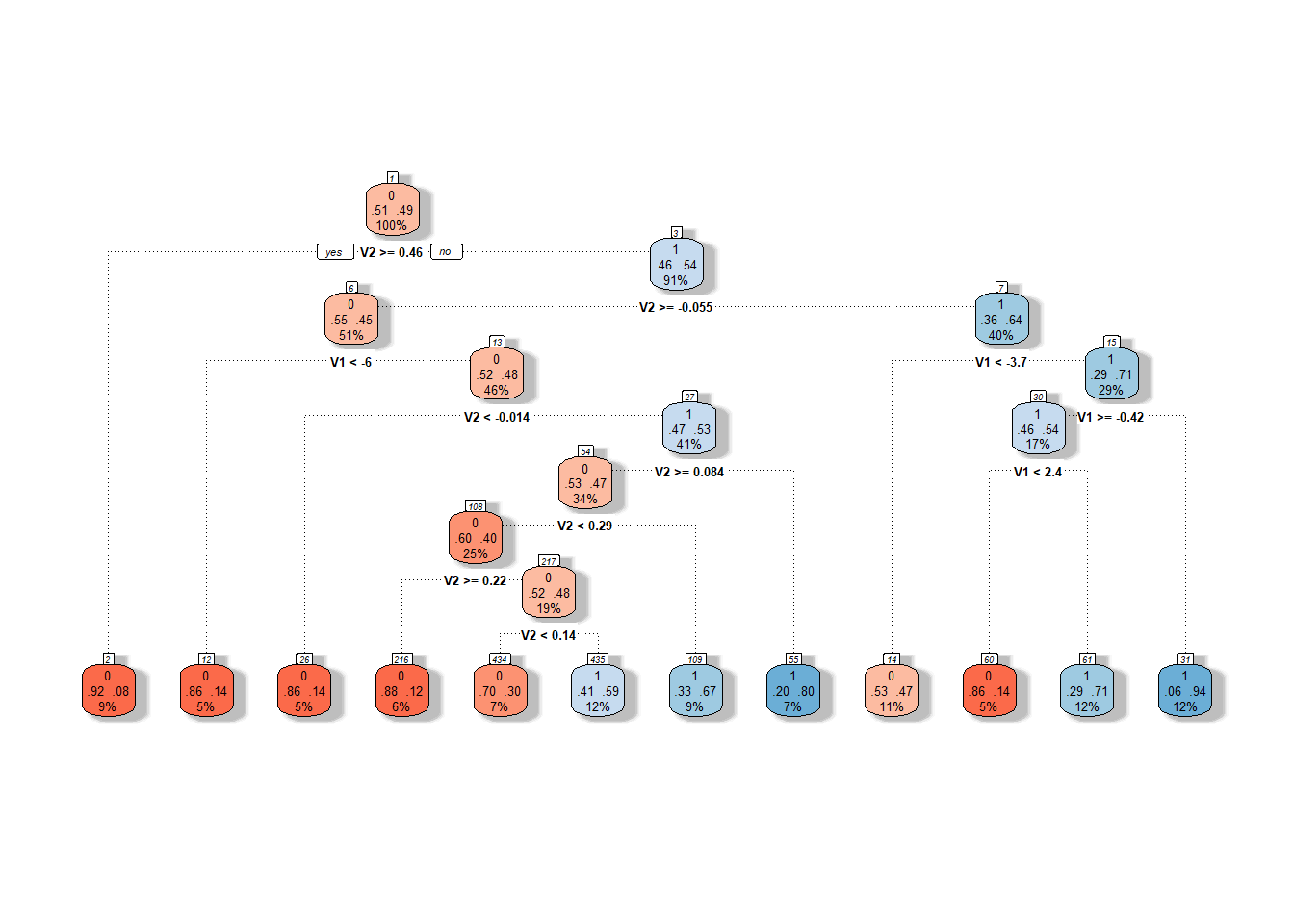
Figure 1.19: Graphic representation of the unpruned decision tree based on principal component scores. Nodes belonging to classification class 1 are shown in blue shades, and those for class 0 are in red shades.

We can also plot the final pruned decision tree.

Code

rpart.plot::rpart.plot(clf.tree.PCA$finalModel, # final model
                       extra = 104, # displaying desired information
                       box.palette = c('Reds', 'Blues'),
                       branch.lty = 3, # dotted branch lines
                       shadow.col = 0, # shadows under the node boxes
                       nn = FALSE, under = FALSE, digits = 2)

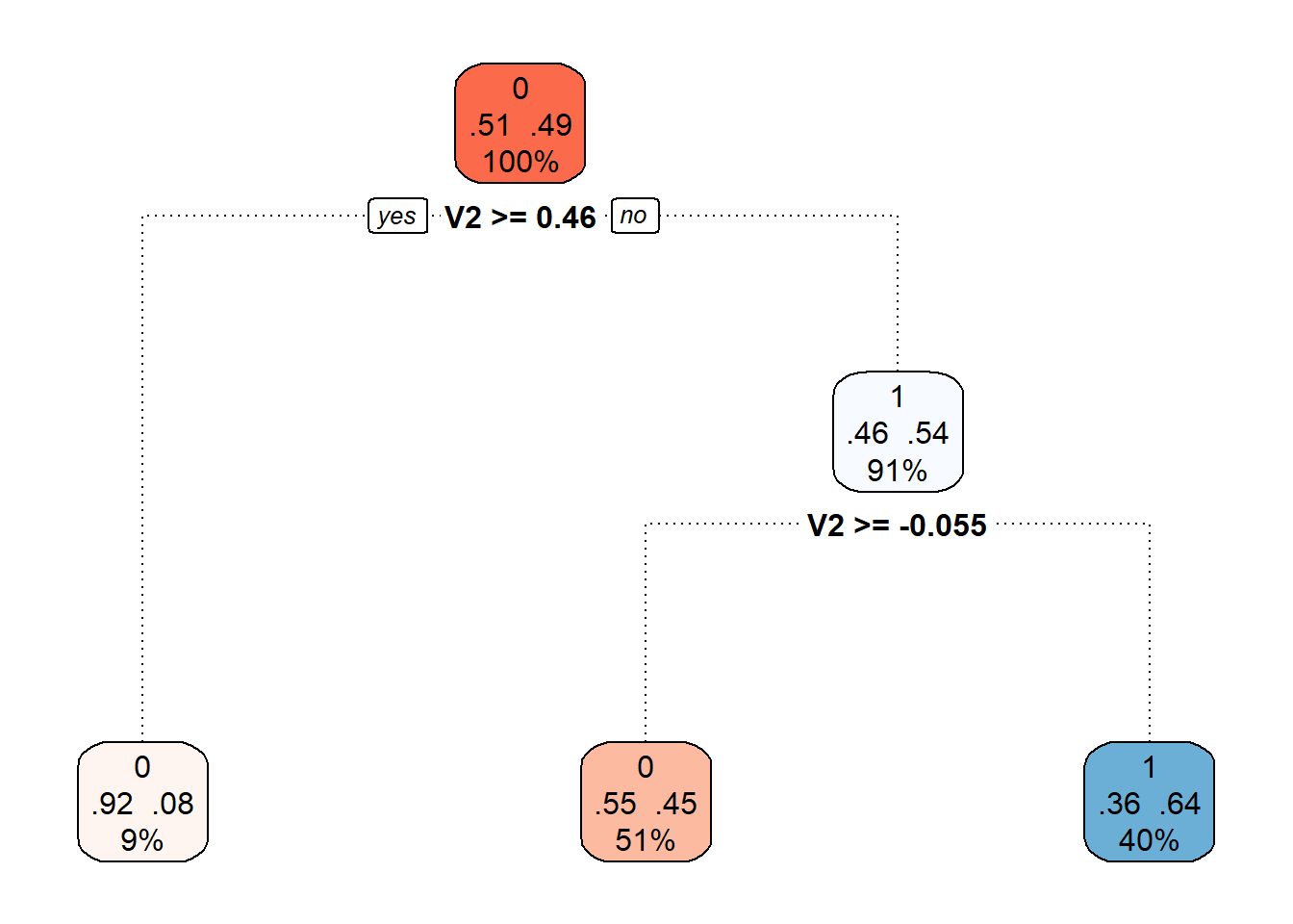
Figure 1.20: Final pruned decision tree.

Finally, we add the training and test error rates to the summary table.

Code

Res <- data.frame(model = 'Tree - score', 
                  Err.train = 1 - accuracy.train,
                  Err.test = 1 - accuracy.test)

RESULTS <- rbind(RESULTS, Res)

1.3.5.3 Basis Coefficients

The final method we will use to construct a decision tree is by employing coefficients derived from the B-spline basis representation of functions.

First, let us define the required datasets with the basis coefficients.

Code

# training dataset
data.Bbasis.train <- t(X.train$coefs) |> as.data.frame()
data.Bbasis.train$Y <- factor(Y.train)

# testing dataset
data.Bbasis.test <- t(X.test$coefs) |> as.data.frame()
data.Bbasis.test$Y <- factor(Y.test)

Now we can proceed to build the classifier.

Code

# model construction
clf.tree.Bbasis <- train(Y ~ ., data = data.Bbasis.train, 
                 method = "rpart", 
                 trControl = trainControl(method = "CV", number = 10),
                 metric = "Accuracy")

# accuracy on training data
predictions.train <- predict(clf.tree.Bbasis, newdata = data.Bbasis.train)
accuracy.train <- table(Y.train, predictions.train) |>
  prop.table() |> diag() |> sum()
  
# accuracy on testing data
predictions.test <- predict(clf.tree.Bbasis, newdata = data.Bbasis.test)
accuracy.test <- table(Y.test, predictions.test) |>
  prop.table() |> diag() |> sum()

The error rate of the decision tree on the training data is 33.57 % and on the testing data 45 %.

We can visualize the decision tree built on the B-spline coefficients using the fancyRpartPlot() function. We set the node colors to reflect the previous color coding. This is an unpruned tree.

Code

fancyRpartPlot(rpart(Y ~ ., data = data.Bbasis.train, method = "class"),
               sub = '', palettes = c('Reds', 'Blues'))

Graphic representation of the unpruned decision tree based on basis coefficients. Nodes belonging to classification class 1 are shown in blue shades, and those for class 0 are in red shades.

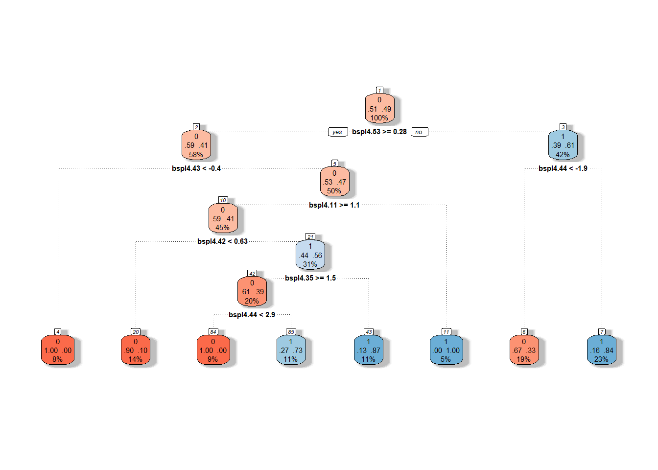
Figure 1.21: Graphic representation of the unpruned decision tree based on basis coefficients. Nodes belonging to classification class 1 are shown in blue shades, and those for class 0 are in red shades.

We can also display the final pruned decision tree.

Code

rpart.plot::rpart.plot(clf.tree.Bbasis$finalModel, # final model
                       extra = 104, # displaying desired information
                       box.palette = c('Reds', 'Blues'),
                       branch.lty = 3, # dotted branch lines
                       shadow.col = 0, # shadows under the node boxes
                       nn = FALSE, under = FALSE, digits = 2)

Figure 1.22: Final pruned decision tree.

Finally, let us add the training and testing error rates to the summary table.

Code

Res <- data.frame(model = 'Tree - Bbasis', 
                  Err.train = 1 - accuracy.train,
                  Err.test = 1 - accuracy.test)

RESULTS <- rbind(RESULTS, Res)

1.3.6 Random Forests

A classifier constructed with the random forest method consists of building multiple individual decision trees that are then combined to form a unified classifier (by “voting” among the trees).

Similar to decision trees, we have several options for which type of (finite-dimensional) data to use in constructing the model. We will once again consider the three approaches discussed above. The datasets with the respective variables for all three approaches have been prepared in the previous section, so we can directly proceed to construct the models, calculate classifier characteristics, and add the results to the summary table.

1.3.6.1 Interval Discretization

In the first case, we evaluate the functions on a specified grid of points in the interval $ I = [0, 6] $.

Code

# model construction
clf.RF <- randomForest(Y ~ ., data = grid.data, 
                       ntree = 500, # number of trees
                       importance = TRUE,
                       nodesize = 5)

# accuracy on training data
predictions.train <- predict(clf.RF, newdata = grid.data)
accuracy.train <- table(Y.train, predictions.train) |>
  prop.table() |> diag() |> sum()
  
# accuracy on testing data
predictions.test <- predict(clf.RF, newdata = grid.data.test)
accuracy.test <- table(Y.test, predictions.test) |>
  prop.table() |> diag() |> sum()

The error rate of the random forest on the training data is 0.71 % and on the testing data 40 %.

Code

Res <- data.frame(model = 'RForest - discr', 
                  Err.train = 1 - accuracy.train,
                  Err.test = 1 - accuracy.test)

RESULTS <- rbind(RESULTS, Res)

1.3.6.2 Principal Component Scores

In this case, we use the scores of the first $ p = $ 2 principal components.

Code

# model construction
clf.RF.PCA <- randomForest(Y ~ ., data = data.PCA.train, 
                           ntree = 500, # number of trees
                           importance = TRUE,
                           nodesize = 5)

# accuracy on training data
predictions.train <- predict(clf.RF.PCA, newdata = data.PCA.train)
accuracy.train <- table(Y.train, predictions.train) |>
  prop.table() |> diag() |> sum()
  
# accuracy on testing data
predictions.test <- predict(clf.RF.PCA, newdata = data.PCA.test)
accuracy.test <- table(Y.test, predictions.test) |>
  prop.table() |> diag() |> sum()

The error rate on the training data is therefore 4.29 % and on the testing data 40 %.

Code

Res <- data.frame(model = 'RForest - score', 
                  Err.train = 1 - accuracy.train,
                  Err.test = 1 - accuracy.test)

RESULTS <- rbind(RESULTS, Res)

1.3.6.3 Basis Coefficients

Finally, we use the function representations through the B-spline basis.

Code

# model construction
clf.RF.Bbasis <- randomForest(Y ~ ., data = data.Bbasis.train, 
                              ntree = 500, # number of trees
                              importance = TRUE,
                              nodesize = 5)

# accuracy on training data
predictions.train <- predict(clf.RF.Bbasis, newdata = data.Bbasis.train)
accuracy.train <- table(Y.train, predictions.train) |>
  prop.table() |> diag() |> sum()
  
# accuracy on testing data
predictions.test <- predict(clf.RF.Bbasis, newdata = data.Bbasis.test)
accuracy.test <- table(Y.test, predictions.test) |>
  prop.table() |> diag() |> sum()

The error rate of this classifier on the training data is 0.71 % and on the testing data 36.67 %.

Code

Res <- data.frame(model = 'RForest - Bbasis', 
                  Err.train = 1 - accuracy.train,
                  Err.test = 1 - accuracy.test)

RESULTS <- rbind(RESULTS, Res)

1.3.7 Support Vector Machines

Now let’s look at the classification of our simulated curves using the Support Vector Machines (SVM) method. The advantage of this classification method is its computational efficiency, as it uses only a few (often very few) observations to define the boundary curve between classes.

The main advantage of SVM is the use of the so-called kernel trick, which allows us to replace the ordinary scalar product with another scalar product of transformed data without having to directly define this transformation. This gives us a generally nonlinear decision boundary between classification classes. The kernel (kernel function) $K$ is a function that satisfies

\[ K(x_i, x_j) = \langle \phi(x_i), \phi(x_j) \rangle_{\mathcal H}, \] where $\phi$ is some (unknown) transformation (feature map), $\mathcal H$ is a Hilbert space, and $\langle \cdot, \cdot \rangle_{\mathcal H}$ is some scalar product in this Hilbert space.

In practice, three types of kernel functions are most commonly chosen:

linear kernel – $K(x_i, x_j) = \langle x_i, x_j \rangle$,
polynomial kernel – $K(x_i, x_j) = \big(\alpha_0 + \gamma \langle x_i, x_j \rangle \big)^d$,
radial (Gaussian) kernel – $\displaystyle{K(x_i, x_j) = \text e^{-\gamma \|x_i - x_j \|^2}}$.

For all the above-mentioned kernels, we must choose a constant $C > 0$, which indicates the degree of penalty for exceeding the decision boundary between classes (inverse regularization parameter). As the value of $C$ increases, the method will penalize poorly classified data more and pay less attention to the shape of the boundary; conversely, for small values of $C$, the method does not give much importance to poorly classified data but focuses more on penalizing the shape of the boundary. This constant $C$ is typically set to 1 by default, but we can also determine it directly, for example, using cross-validation.

By using cross-validation, we can also determine the optimal values of other hyperparameters, which now depend on our choice of kernel function. In the case of a linear kernel, we do not choose any other parameters aside from the constant $C$; with polynomial and radial kernels, we must specify the hyperparameter values $\alpha_0, \gamma, \text{ and } d$, whose default values in R are sequentially $\alpha_0^{default} = 0, \gamma^{default} = \frac{1}{\text{dim}(\texttt{data})} \text{ and } d^{default} = 3$. Again, we could determine the optimal hyperparameter values for our data, but due to the relatively high computational cost, we will leave the values of the respective hyperparameters at the values estimated using CV on a generated dataset, choosing $\alpha_0 = 1$.

In the case of functional data, we have several options for applying the SVM method. The simplest variant is to apply this classification method directly to the discretized function (section 1.3.7.2). Another option is to again use the principal component scores and classify the curves based on their representation 1.3.7.3. Another straightforward variant is to utilize the expression of curves using a B-spline basis and classify the curves based on the coefficients of their representation in this basis (section 1.3.7.4).

Through more complex reasoning, we can arrive at several other options that utilize the functional nature of the data. On the one hand, instead of classifying the original curve, we can use its derivative (or second derivative, third, etc.); on the other hand, we can utilize the projection of functions onto the subspace generated by, for example, B-spline functions (section 1.3.7.5). The last method we will use for classifying functional data involves a combination of projecting onto a certain subspace generated by functions (Reproducing Kernel Hilbert Space, RKHS) and classifying the corresponding representation. This method utilizes both classical SVM and SVM for regression; more details can be found in the section RKHS + SVM 1.3.7.6.

1.3.7.1 SVM for Functional Data

In the fda.usc library, we will use the function classif.svm() to apply the SVM method directly to functional data. First, we will create suitable objects for constructing the classifier.

Code

# set norm equal to one
norms <- c()
for (i in 1:dim(XXfd$coefs)[2]) {
  norms <- c(norms, as.numeric(1 / norm.fd(XXfd[i])))
}
XXfd_norm <- XXfd 
XXfd_norm$coefs <- XXfd_norm$coefs * matrix(norms, 
    ncol = dim(XXfd$coefs)[2],
    nrow = dim(XXfd$coefs)[1],
    byrow = T)

# splitting into test and training parts
X.train_norm <- subset(XXfd_norm, split == TRUE)
X.test_norm <- subset(XXfd_norm, split == FALSE)

Y.train_norm <- subset(Y, split == TRUE)
Y.test_norm <- subset(Y, split == FALSE)

Code

# create suitable objects
x.train <- fdata(X.train_norm)
y.train <- as.factor(Y.train_norm)

# points at which the functions are evaluated
tt <- x.train[["argvals"]]

dataf <- as.data.frame(y.train) 
colnames(dataf) <- "Y"
# B-spline basis 
basis1 <- X.train_norm$basis

Code

# formula
f <- Y ~ x 
# basis for x
basis.x <- list("x" = basis1) 
# input data for the model
ldata <- list("df" = dataf, "x" = x.train)
# SVM model
model.svm.f <- classif.svm(formula = f,
            data = ldata,
            basis.x = basis.x,
            kernel = 'polynomial', degree = 5, coef0 = 1, cost = 1e4)

# accuracy on training data
newdat <- list("x" = x.train)
predictions.train <- predict(model.svm.f, newdat, type = 'class')
presnost.train <- mean(factor(Y.train_norm) == predictions.train)
  
# accuracy on test data
newdat <- list("x" = fdata(X.test_norm))
predictions.test <- predict(model.svm.f, newdat, type = 'class')
presnost.test <- mean(factor(Y.test_norm) == predictions.test)

We calculated the training error (which is 0 %) and the test error (which is 11.67 %).

Now let’s attempt, unlike the procedure in the previous chapters, to estimate the hyperparameters of the classifiers from the data using 10-fold cross-validation. Since each kernel has different hyperparameters in its definition, we will approach each kernel function separately. However, the hyperparameter $C$ appears in all kernel functions, acknowledging that its optimal value may differ between kernels.

For all three kernels, we will explore the values of the hyperparameter $C$ in the range $[10^{0}, 10^{7}]$, while for the polynomial kernel, we will consider the value of the hyperparameter $p$ to be 3, 4, or 5, as other integer values do not yield nearly as good results. Conversely, for the radial kernel, we will again use $r k_cv$-fold CV to choose the optimal value of the hyperparameter $\gamma$, considering values in the range $[10^{-5}, 10^{0}]$. We will set coef0 to 1.

Code

set.seed(42)

k_cv <- 10 #  k-fold CV

# We split the training data into k parts
folds <- createMultiFolds(1:sum(split), k = k_cv, time = 1)

# Which values of gamma do we want to consider
gamma.cv <- 10^seq(-5, 0, length = 6)
C.cv <- 10^seq(0, 7, length = 8)
p.cv <- c(3, 4, 5)
coef0 <- 1

# A list with three components... an array for each kernel -> linear, poly, radial
# An empty matrix where we will place individual results
# The columns will contain the accuracy values for each
# The rows will correspond to the values for a given gamma and the layers correspond to folds
CV.results <- list(
  SVM.l = array(NA, dim = c(length(C.cv), k_cv)),
  SVM.p = array(NA, dim = c(length(C.cv), length(p.cv), k_cv)),
  SVM.r = array(NA, dim = c(length(C.cv), length(gamma.cv), k_cv))
)

# First, we go through the values of C
for (cost in C.cv) {
  # We go through the individual folds
  for (index_cv in 1:k_cv) {
    # Definition of the test and training parts for CV
    fold <- folds[[index_cv]]
    cv_sample <- 1:dim(X.train_norm$coefs)[2] %in% fold
    
    x.train.cv <- fdata(subset(X.train_norm, cv_sample))
    x.test.cv <- fdata(subset(X.train_norm, !cv_sample))
    y.train.cv <- as.factor(subset(Y.train_norm, cv_sample))
    y.test.cv <- as.factor(subset(Y.train_norm, !cv_sample))
    
    # Points at which the functions are evaluated
    tt <- x.train.cv[["argvals"]]
    
    dataf <- as.data.frame(y.train.cv) 
    colnames(dataf) <- "Y"
    # B-spline basis
    basis1 <- X.train_norm$basis
    # Formula
    f <- Y ~ x 
    # Basis for x
    basis.x <- list("x" = basis1) 
    # Input data for the model
    ldata <- list("df" = dataf, "x" = x.train.cv)
    
    ## LINEAR KERNEL
    # SVM model
    clf.svm.f_l <- classif.svm(formula = f,
                data = ldata,
                basis.x = basis.x,
                kernel = 'linear',
                cost = cost,
                type = 'C-classification',
                scale = TRUE)
      
    # Accuracy on the test data
    newdat <- list("x" = x.test.cv)
    predictions.test <- predict(clf.svm.f_l, newdat, type = 'class')
    accuracy.test.l <- mean(y.test.cv == predictions.test)
    
    # We insert the accuracies into positions for the given C and fold
    CV.results$SVM.l[(1:length(C.cv))[C.cv == cost], 
                     index_cv] <- accuracy.test.l
    
    ## POLYNOMIAL KERNEL
    for (p in p.cv) {
      # Model construction
      clf.svm.f_p <- classif.svm(formula = f,
                data = ldata,
                basis.x = basis.x,
                kernel = 'polynomial',
                cost = cost,
                coef0 = coef0,
                degree = p,
                type = 'C-classification',
                scale = TRUE)
        
      # Accuracy on the test data
      newdat <- list("x" = x.test.cv)
      predictions.test <- predict(clf.svm.f_p, newdat, type = 'class')
      accuracy.test.p <- mean(y.test.cv == predictions.test)
      
      # We insert the accuracies into positions for the given C, p, and fold
      CV.results$SVM.p[(1:length(C.cv))[C.cv == cost], 
                       (1:length(p.cv))[p.cv == p],
                       index_cv] <- accuracy.test.p
    }
        
    ## RADIAL KERNEL
    for (gam.cv in gamma.cv) {
      # Model construction
      clf.svm.f_r <- classif.svm(formula = f,
                data = ldata,
                basis.x = basis.x,
                kernel = 'radial',
                cost = cost,
                gamma = gam.cv,
                type = 'C-classification',
                scale = TRUE)
        
      # Accuracy on the test data
      newdat <- list("x" = x.test.cv)
      predictions.test <- predict(clf.svm.f_r, newdat, type = 'class')
      accuracy.test.r <- mean(y.test.cv == predictions.test)
      
      # We insert the accuracies into positions for the given C, gamma, and fold
      CV.results$SVM.r[(1:length(C.cv))[C.cv == cost], 
                       (1:length(gamma.cv))[gamma.cv == gam.cv],
                       index_cv] <- accuracy.test.r
    }
  }
}

Now we will average the results of 10-fold CV so that we have one estimate of validation error for one value of the hyperparameter (or one combination of values). At the same time, we will determine the optimal values of the individual hyperparameters.

Code

# We calculate the average accuracies for individual C across folds
## Linear kernel
CV.results$SVM.l <- apply(CV.results$SVM.l, 1, mean)
## Polynomial kernel
CV.results$SVM.p <- apply(CV.results$SVM.p, c(1, 2), mean)
## Radial kernel
CV.results$SVM.r <- apply(CV.results$SVM.r, c(1, 2), mean)

C.opt <- c(which.max(CV.results$SVM.l), 
           which.max(CV.results$SVM.p) %% length(C.cv), 
           which.max(CV.results$SVM.r) %% length(C.cv))
C.opt[C.opt == 0] <- length(C.cv)
C.opt <- C.cv[C.opt]

gamma.opt <- which.max(t(CV.results$SVM.r)) %% length(gamma.cv)
gamma.opt[gamma.opt == 0] <- length(gamma.cv)
gamma.opt <- gamma.cv[gamma.opt]

p.opt <- which.max(t(CV.results$SVM.p)) %% length(p.cv)
p.opt[p.opt == 0] <- length(p.cv)
p.opt <- p.cv[p.opt]

accuracy.opt.cv <- c(max(CV.results$SVM.l), 
                     max(CV.results$SVM.p),
                     max(CV.results$SVM.r))

Let’s take a look at how the optimal values turned out. For linear kernel, we have the optimal value $C$ equal to 100, for polynomial kernel $C$ is equal to 1, and for radial kernel, we have two optimal values, for $C$ the optimal value is 10^{6} and for $\gamma$ it is 10^{-4}. The validation error rates are 0.0935256 for linear, 0.1731822 for polynomial, and 0.0787637 for radial kernel.

Finally, we can construct the final classifiers on the entire training data with the hyperparameter values determined using 10-fold CV. We will also determine the errors on the test and training data.

Code

# Create suitable objects
x.train <- fdata(X.train_norm)
y.train <- as.factor(Y.train_norm)

# Points at which the functions are evaluated
tt <- x.train[["argvals"]]

dataf <- as.data.frame(y.train) 
colnames(dataf) <- "Y"
# B-spline basis
basis1 <- X.train_norm$basis

# Formula
f <- Y ~ x 
# Basis for x
basis.x <- list("x" = basis1) 
# Input data for the model
ldata <- list("df" = dataf, "x" = x.train)

Code

model.svm.f_l <- classif.svm(formula = f,
            data = ldata,
            basis.x = basis.x,
            kernel = 'linear', 
            type = 'C-classification',
            scale = TRUE,
            cost = C.opt[1])

model.svm.f_p <- classif.svm(formula = f,
            data = ldata,
            basis.x = basis.x,
            kernel = 'polynomial', 
            type = 'C-classification',
            scale = TRUE,
            degree = p.opt,
            coef0 = coef0,
            cost = C.opt[2])

model.svm.f_r <- classif.svm(formula = f,
            data = ldata,
            basis.x = basis.x,
            kernel = 'radial', 
            type = 'C-classification',
            scale = TRUE,
            gamma = gamma.opt,
            cost = C.opt[3])

# Accuracy on training data
newdat <- list("x" = x.train)
predictions.train.l <- predict(model.svm.f_l, newdat, type = 'class')
accuracy.train.l <- mean(factor(Y.train_norm) == predictions.train.l)

predictions.train.p <- predict(model.svm.f_p, newdat, type = 'class')
accuracy.train.p <- mean(factor(Y.train_norm) == predictions.train.p)

predictions.train.r <- predict(model.svm.f_r, newdat, type = 'class')
accuracy.train.r <- mean(factor(Y.train_norm) == predictions.train.r)
  
# Accuracy on test data
newdat <- list("x" = fdata(X.test_norm))
predictions.test.l <- predict(model.svm.f_l, newdat, type = 'class')
accuracy.test.l <- mean(factor(Y.test_norm) == predictions.test.l)

predictions.test.p <- predict(model.svm.f_p, newdat, type = 'class')
accuracy.test.p <- mean(factor(Y.test_norm) == predictions.test.p)

predictions.test.r <- predict(model.svm.f_r, newdat, type = 'class')
accuracy.test.r <- mean(factor(Y.test_norm) == predictions.test.r)

The error rate of the SVM method on the training data is thus 5 % for the linear kernel, 11.4286 % for the polynomial kernel, and 2.8571 % for the Gaussian kernel. On the test data, the error rate of the method is 23.3333 % for the linear kernel, 26.6667 % for the polynomial kernel, and 13.3333 % for the radial kernel.

Code

Res <- data.frame(model = c('SVM linear - func', 
                            'SVM poly - func', 
                            'SVM rbf - func'), 
                  Err.train = 1 - c(accuracy.train.l, accuracy.train.p, accuracy.train.r),
                  Err.test = 1 - c(accuracy.test.l, accuracy.test.p, accuracy.test.r))

RESULTS <- rbind(RESULTS, Res)

1.3.7.2 Discretization of the Interval

Let’s start by applying the support vector method directly to the discretized data (evaluating the function on a given grid of points over the interval $I = [0, 6]$), considering all three aforementioned kernel functions.

Code

# Set norms equal to one
norms <- c()
for (i in 1:dim(XXfd$coefs)[2]) {
  norms <- c(norms, as.numeric(1 / norm.fd(XXfd[i])))
}
XXfd_norm <- XXfd 
XXfd_norm$coefs <- XXfd_norm$coefs * matrix(norms, 
                                            ncol = dim(XXfd$coefs)[2],
                                            nrow = dim(XXfd$coefs)[1],
                                            byrow = TRUE)

# Split into test and training parts
X.train_norm <- subset(XXfd_norm, split == TRUE)
X.test_norm <- subset(XXfd_norm, split == FALSE)

Y.train_norm <- subset(Y, split == TRUE)
Y.test_norm <- subset(Y, split == FALSE)

grid.data <- eval.fd(fdobj = X.train_norm, evalarg = t.seq)
grid.data <- as.data.frame(t(grid.data)) 
grid.data$Y <- Y.train_norm |> factor()

grid.data.test <- eval.fd(fdobj = X.test_norm, evalarg = t.seq)
grid.data.test <- as.data.frame(t(grid.data.test))
grid.data.test$Y <- Y.test_norm |> factor()

Now, let’s attempt to estimate the hyperparameters of the classifiers from the data using 10-fold cross-validation. Since each kernel has different hyperparameters in its definition, we will approach each kernel function separately. However, the hyperparameter $C$ appears in all kernel functions, and we allow its optimal value to differ among kernels.

For all three kernels, we will go through the values of the hyperparameter $C$ in the interval $[10^{0}, 10^{6}]$, while for the polynomial kernel we will fix the hyperparameter $p$ at a value of 3, since other integer values do not yield nearly as good results. On the other hand, for the radial kernel, we will use 10-fold CV to choose the optimal value of the hyperparameter $\gamma$, considering values in the interval $[10^{-5}, 10^{-2}]$. We will set coef0 to 1.

Code

set.seed(42)

k_cv <- 10 # k-fold CV

# Split training data into k parts
folds <- createMultiFolds(1:sum(split), k = k_cv, time = 1)

# Values of gamma to consider
gamma.cv <- 10^seq(-5, -2, length = 7)
C.cv <- 10^seq(0, 6, length = 7)
p.cv <- 3
coef0 <- 1

# List with three components ... arrays for individual kernels -> linear, poly, radial
# Empty matrices to store the results
# Columns will contain accuracy values for given C
# Rows will contain values for given gamma, and layers correspond to folds
CV.results <- list(
  SVM.l = array(NA, dim = c(length(C.cv), k_cv)),
  SVM.p = array(NA, dim = c(length(C.cv), length(p.cv), k_cv)),
  SVM.r = array(NA, dim = c(length(C.cv), length(gamma.cv), k_cv))
)

# First, we go through the values of C
for (C in C.cv) {
  # Go through individual folds
  for (index_cv in 1:k_cv) {
    # Definition of test and training parts for CV
    fold <- folds[[index_cv]]
    cv_sample <- 1:dim(grid.data)[1] %in% fold
    
    data.grid.train.cv <- as.data.frame(grid.data[cv_sample, ])
    data.grid.test.cv <- as.data.frame(grid.data[!cv_sample, ])
    
    ## LINEAR KERNEL
    # Model construction
    clf.SVM.l <- svm(Y ~ ., data = data.grid.train.cv,
                     type = 'C-classification',
                     scale = TRUE,
                     cost = C,
                     kernel = 'linear')
    
    # Accuracy on validation data
    predictions.test.l <- predict(clf.SVM.l, newdata = data.grid.test.cv)
    accuracy.test.l <- table(data.grid.test.cv$Y, predictions.test.l) |>
      prop.table() |> diag() |> sum()
    
    # Store accuracy for given C and fold
    CV.results$SVM.l[(1:length(C.cv))[C.cv == C], 
                     index_cv] <- accuracy.test.l
    
    ## POLYNOMIAL KERNEL
    for (p in p.cv) {
      # Model construction
      clf.SVM.p <- svm(Y ~ ., data = data.grid.train.cv,
                       type = 'C-classification',
                       scale = TRUE,
                       cost = C,
                       coef0 = coef0,
                       degree = p,
                       kernel = 'polynomial')
      
      # Accuracy on validation data
      predictions.test.p <- predict(clf.SVM.p, newdata = data.grid.test.cv)
      accuracy.test.p <- table(data.grid.test.cv$Y, predictions.test.p) |>
        prop.table() |> diag() |> sum()
      
      # Store accuracy for given C, p, and fold
      CV.results$SVM.p[(1:length(C.cv))[C.cv == C], 
                       (1:length(p.cv))[p.cv == p],
                       index_cv] <- accuracy.test.p
    }
        
    ## RADIAL KERNEL
    for (gamma in gamma.cv) {
      # Model construction
      clf.SVM.r <- svm(Y ~ ., data = data.grid.train.cv,
                       type = 'C-classification',
                       scale = TRUE,
                       cost = C,
                       gamma = gamma,
                       kernel = 'radial')
      
      # Accuracy on validation data
      predictions.test.r <- predict(clf.SVM.r, newdata = data.grid.test.cv)
      accuracy.test.r <- table(data.grid.test.cv$Y, predictions.test.r) |>
        prop.table() |> diag() |> sum()
      
      # Store accuracy for given C, gamma, and fold
      CV.results$SVM.r[(1:length(C.cv))[C.cv == C], 
                       (1:length(gamma.cv))[gamma.cv == gamma],
                       index_cv] <- accuracy.test.r
    }
  }
}

Now, let’s average the results of the 10-fold CV so that for each value of the hyperparameter (or one combination of values), we have one estimate of the validation error. In this process, we will also determine the optimal values for the individual hyperparameters.

Code

# Calculate average accuracies for each C across folds
## Linear kernel
CV.results$SVM.l <- apply(CV.results$SVM.l, 1, mean)
## Polynomial kernel
CV.results$SVM.p <- apply(CV.results$SVM.p, c(1, 2), mean)
## Radial kernel
CV.results$SVM.r <- apply(CV.results$SVM.r, c(1, 2), mean)

C.opt <- c(which.max(CV.results$SVM.l), 
           which.max(CV.results$SVM.p) %% length(C.cv), 
           which.max(CV.results$SVM.r) %% length(C.cv))
C.opt[C.opt == 0] <- length(C.cv)
C.opt <- C.cv[C.opt]

gamma.opt <- which.max(t(CV.results$SVM.r)) %% length(gamma.cv)
gamma.opt[gamma.opt == 0] <- length(gamma.cv)
gamma.opt <- gamma.cv[gamma.opt]

p.opt <- which.max(t(CV.results$SVM.p)) %% length(p.cv)
p.opt[p.opt == 0] <- length(p.cv)
p.opt <- p.cv[p.opt]

accuracy.opt.cv <- c(max(CV.results$SVM.l), 
                     max(CV.results$SVM.p),
                     max(CV.results$SVM.r))

Let’s look at how the optimal values turned out. For the linear kernel, the optimal value of $C$ is 100, for the polynomial kernel $C$ is 10, and for the radial kernel, we have two optimal values: for $C$, the optimal value is 10^{6}, and for $\gamma$, it is 0. The validation errors are 0.0875733 for linear, 0.160815 for polynomial, and 0.0859066 for radial kernels.

Finally, we can construct the final classifiers on the entire training data with the hyperparameter values determined by 10-fold CV. We will also determine the errors on both test and training datasets.

Code

# Model construction
clf.SVM.l <- svm(Y ~ ., data = grid.data,
                 type = 'C-classification',
                 scale = TRUE,
                 cost = C.opt[1],
                 kernel = 'linear')

clf.SVM.p <- svm(Y ~ ., data = grid.data,
                 type = 'C-classification',
                 scale = TRUE,
                 cost = C.opt[2],
                 degree = p.opt,
                 coef0 = coef0,
                 kernel = 'polynomial')

clf.SVM.r <- svm(Y ~ ., data = grid.data,
                 type = 'C-classification',
                 scale = TRUE, 
                 cost = C.opt[3],
                 gamma = gamma.opt,
                 kernel = 'radial')

# Accuracy on training data
predictions.train.l <- predict(clf.SVM.l, newdata = grid.data)
accuracy.train.l <- table(Y.train, predictions.train.l) |>
  prop.table() |> diag() |> sum()

predictions.train.p <- predict(clf.SVM.p, newdata = grid.data)
accuracy.train.p <- table(Y.train, predictions.train.p) |>
  prop.table() |> diag() |> sum()

predictions.train.r <- predict(clf.SVM.r, newdata = grid.data)
accuracy.train.r <- table(Y.train, predictions.train.r) |>
  prop.table() |> diag() |> sum()

# Accuracy on test data
predictions.test.l <- predict(clf.SVM.l, newdata = grid.data.test)
accuracy.test.l <- table(Y.test, predictions.test.l) |>
  prop.table() |> diag() |> sum()

predictions.test.p <- predict(clf.SVM.p, newdata = grid.data.test)
accuracy.test.p <- table(Y.test, predictions.test.p) |>
  prop.table() |> diag() |> sum()

predictions.test.r <- predict(clf.SVM.r, newdata = grid.data.test)
accuracy.test.r <- table(Y.test, predictions.test.r) |>
  prop.table() |> diag() |> sum()

The error rate of the SVM method on the training data is 5.7143 % for the linear kernel, 9.2857 % for the polynomial kernel, and 2.1429 % for the Gaussian kernel. On the test data, the error rate is 16.6667 % for the linear kernel, 21.6667 % for the polynomial kernel, and 11.6667 % for the radial kernel.

Code

Res <- data.frame(model = c('SVM linear - discr', 
                            'SVM poly - discr', 
                            'SVM rbf - discr'), 
                  Err.train = 1 - c(accuracy.train.l, accuracy.train.p, accuracy.train.r),
                  Err.test = 1 - c(accuracy.test.l, accuracy.test.p, accuracy.test.r))

RESULTS <- rbind(RESULTS, Res)

1.3.7.3 Principal Component Scores

In this case, we use the scores of the first $p =$ 2 principal components.

Now, let’s try, unlike the approach in previous chapters, to estimate the classifier hyperparameters from the data using 10-fold cross-validation. Given that each kernel has different hyperparameters in its definition, we will treat each kernel function separately. However, the hyperparameter $C$ appears in all kernel functions, although we allow that its optimal value may differ between kernels.

For all three kernels, we will test values of the hyperparameter $C$ in the interval $[10^{-3}, 10^{4}]$. For the polynomial kernel, we fix the hyperparameter $p$ at the value of 3, as for other integer values, the method does not give nearly as good results. In contrast, for the radial kernel, we will use 10-fold CV to choose the optimal value of the hyperparameter $\gamma$, considering values in the interval $[10^{-4}, 10^{-1}]$. We set coef0 $= 1$.

Code

set.seed(42)

# gamma values to consider
gamma.cv <- 10^seq(-4, -1, length = 7)
C.cv <- 10^seq(-3, 4, length = 8)
p.cv <- 3
coef0 <- 1

# list with three components ... array for individual kernels -> linear, poly, radial
# empty matrix to store results
# columns will have accuracy values for a given
# rows will have values for given gamma and layers correspond to folds
CV.results <- list(
  SVM.l = array(NA, dim = c(length(C.cv), k_cv)),
  SVM.p = array(NA, dim = c(length(C.cv), length(p.cv), k_cv)),
  SVM.r = array(NA, dim = c(length(C.cv), length(gamma.cv), k_cv))
)

# first, go through C values
for (C in C.cv) {
  # iterate over each fold
  for (index_cv in 1:k_cv) {
    # define test and training parts for CV
    fold <- folds[[index_cv]]
    cv_sample <- 1:dim(data.PCA.train)[1] %in% fold
    
    data.PCA.train.cv <- as.data.frame(data.PCA.train[cv_sample, ])
    data.PCA.test.cv <- as.data.frame(data.PCA.train[!cv_sample, ])
    
    ## LINEAR KERNEL
    # build model
    clf.SVM.l <- svm(Y ~ ., data = data.PCA.train.cv,
                     type = 'C-classification',
                     scale = TRUE,
                     cost = C,
                     kernel = 'linear')
    
    # accuracy on validation data
    predictions.test.l <- predict(clf.SVM.l, newdata = data.PCA.test.cv)
    presnost.test.l <- table(data.PCA.test.cv$Y, predictions.test.l) |>
      prop.table() |> diag() |> sum()
    
    # store accuracies for given C and fold
    CV.results$SVM.l[(1:length(C.cv))[C.cv == C], 
                     index_cv] <- presnost.test.l
    
    ## POLYNOMIAL KERNEL
    for (p in p.cv) {
      # build model
      clf.SVM.p <- svm(Y ~ ., data = data.PCA.train.cv,
                       type = 'C-classification',
                       scale = TRUE,
                       cost = C,
                       coef0 = coef0,
                       degree = p,
                       kernel = 'polynomial')
      
      # accuracy on validation data
      predictions.test.p <- predict(clf.SVM.p, newdata = data.PCA.test.cv)
      presnost.test.p <- table(data.PCA.test.cv$Y, predictions.test.p) |>
        prop.table() |> diag() |> sum()
      
      # store accuracies for given C, p, and fold
      CV.results$SVM.p[(1:length(C.cv))[C.cv == C], 
                       (1:length(p.cv))[p.cv == p],
                       index_cv] <- presnost.test.p
    }
        
    ## RADIAL KERNEL
    for (gamma in gamma.cv) {
      # build model
      clf.SVM.r <- svm(Y ~ ., data = data.PCA.train.cv,
                       type = 'C-classification',
                       scale = TRUE,
                       cost = C,
                       gamma = gamma,
                       kernel = 'radial')
      
      # accuracy on validation data
      predictions.test.r <- predict(clf.SVM.r, newdata = data.PCA.test.cv)
      presnost.test.r <- table(data.PCA.test.cv$Y, predictions.test.r) |>
        prop.table() |> diag() |> sum()
      
      # store accuracies for given C, gamma, and fold
      CV.results$SVM.r[(1:length(C.cv))[C.cv == C], 
                       (1:length(gamma.cv))[gamma.cv == gamma],
                       index_cv] <- presnost.test.r
    }
  }
}

Now we average the results of the 10-fold CV to obtain a single estimate of validation error for each hyperparameter value (or combination of values). We also determine the optimal values of each hyperparameter.

Code

# calculate average accuracies for individual C over folds
## Linear kernel
CV.results$SVM.l <- apply(CV.results$SVM.l, 1, mean)
## Polynomial kernel
CV.results$SVM.p <- apply(CV.results$SVM.p, c(1, 2), mean)
## Radial kernel
CV.results$SVM.r <- apply(CV.results$SVM.r, c(1, 2), mean)

C.opt <- c(which.max(CV.results$SVM.l), 
           which.max(CV.results$SVM.p) %% length(C.cv), 
           which.max(CV.results$SVM.r) %% length(C.cv))
C.opt[C.opt == 0] <- length(C.cv)
C.opt <- C.cv[C.opt]

gamma.opt <- which.max(t(CV.results$SVM.r)) %% length(gamma.cv)
gamma.opt[gamma.opt == 0] <- length(gamma.cv)
gamma.opt <- gamma.cv[gamma.opt]

p.opt <- which.max(t(CV.results$SVM.p)) %% length(p.cv)
p.opt[p.opt == 0] <- length(p.cv)
p.opt <- p.cv[p.opt]

presnost.opt.cv <- c(max(CV.results$SVM.l), 
                     max(CV.results$SVM.p),
                     max(CV.results$SVM.r))

Let’s look at how the optimal values turned out. For the linear kernel, the optimal value of $C$ is 10, for the polynomial kernel $C$ is 0.01, and for the radial kernel, there are two optimal values: $C$ is 10^{4} and $\gamma$ is 0.001. The validation errors are 0.4097253 for linear, 0.4287454 for polynomial, and 0.3906502 for the radial kernel.

Finally, we can construct the final classifiers on the entire training dataset with hyperparameter values determined using 10-fold CV. We also calculate errors on the test and training datasets.

Code

# build model
clf.SVM.l.PCA <- svm(Y ~ ., data = data.PCA.train,
                     type = 'C-classification',
                     scale = TRUE,
                     cost = C.opt[1],
                     kernel = 'linear')

clf.SVM.p.PCA <- svm(Y ~ ., data = data.PCA.train,
                     type = 'C-classification',
                     scale = TRUE,
                     cost = C.opt[2],
                     degree = p.opt,
                     coef0 = coef0,
                     kernel = 'polynomial')

clf.SVM.r.PCA <- svm(Y ~ ., data = data.PCA.train,
                     type = 'C-classification',
                     scale = TRUE,
                     cost = C.opt[3],
                     gamma = gamma.opt,
                     kernel = 'radial')

# accuracy on training data
predictions.train.l <- predict(clf.SVM.l.PCA, newdata = data.PCA.train)
presnost.train.l <- table(data.PCA.train$Y, predictions.train.l) |>
  prop.table() |> diag() |> sum()

predictions.train.p <- predict(clf.SVM.p.PCA, newdata = data.PCA.train)
presnost.train.p <- table(data.PCA.train$Y, predictions.train.p) |>
  prop.table() |> diag() |> sum()

predictions.train.r <- predict(clf.SVM.r.PCA, newdata = data.PCA.train)
presnost.train.r <- table(data.PCA.train$Y, predictions.train.r) |>
  prop.table() |> diag() |> sum()
  
# accuracy on test data
predictions.test.l <- predict(clf.SVM.l.PCA, newdata = data.PCA.test)
presnost.test.l <- table(data.PCA.test$Y, predictions.test.l) |>
  prop.table() |> diag() |> sum()

predictions.test.p <- predict(clf.SVM.p.PCA, newdata = data.PCA.test)
presnost.test.p <- table(data.PCA.test$Y, predictions.test.p) |>
  prop.table() |> diag() |> sum()

predictions.test.r <- predict(clf.SVM.r.PCA, newdata = data.PCA.test)
presnost.test.r <- table(data.PCA.test$Y, predictions.test.r) |>
  prop.table() |> diag() |> sum()

The training accuracies are 0.6 for linear, 0.5928571 for polynomial, and 0.6357143 for radial kernels, and the test accuracies are 0.6 for linear, 0.6 for polynomial, and 0.5833333 for radial.

To visualize the method, we can plot the decision boundary on a graph of the scores for the first two principal components. We compute this boundary on a dense grid of points and display it using the geom_contour() function, just as in previous cases where we also plotted the classification boundary.

Code

nd <- rbind(nd, nd, nd) |> mutate(
   prd = c(as.numeric(predict(clf.SVM.l.PCA, newdata = nd, type = 'response')),
           as.numeric(predict(clf.SVM.p.PCA, newdata = nd, type = 'response')),
           as.numeric(predict(clf.SVM.r.PCA, newdata = nd, type = 'response'))),
   kernel = rep(c('linear', 'polynomial', 'radial'),
                each = length(as.numeric(predict(clf.SVM.l.PCA, 
                                                 newdata = nd,
                                                 type = 'response')))) |>
     as.factor())

data.PCA.train |> ggplot(aes(x = V1, y = V2, colour = Y)) +
 geom_point(size = 1.5) + 
 labs(x = paste('1st Principal Component (Explained Variance', 
                round(100 * data.PCA$varprop[1], 2), '%)'),
      y = paste('2nd Principal Component (', 
                round(100 * data.PCA$varprop[2], 2), '%)'),
      colour = 'Fat Content', 
      linetype = 'Kernel') +
 scale_colour_discrete(labels = c("low", "high")) +
 theme_bw() +
 geom_contour(data = nd, aes(x = V1, y = V2, z = prd, linetype = kernel), 
              colour = 'black')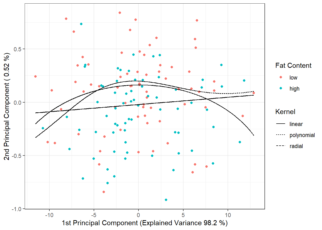

Figure 1.23: Scores of the first two principal components, color-coded by classification group. The decision boundary (either a line or curves in the plane of the first two principal components) between classes is displayed in black, created using the SVM method.

Code

Res <- data.frame(model = c('SVM linear - PCA', 
                            'SVM poly - PCA', 
                            'SVM rbf - PCA'), 
                  Err.train = 1 - c(presnost.train.l, presnost.train.p, presnost.train.r),
                  Err.test = 1 - c(presnost.test.l, presnost.test.p, presnost.test.r))

RESULTS <- rbind(RESULTS, Res)

1.3.7.4 Basis Coefficients

Finally, we use a B-spline basis to express the functions. For all three kernels, we examine the values of hyperparameter $C$ in the interval $[10^{1}, 10^{4}]$. For the polynomial kernel, we fix the hyperparameter $p$ at 3, as other integer values do not yield nearly as good results. On the other hand, for the radial kernel, we again use 10-fold CV to select the optimal value of hyperparameter $\gamma$, considering values in the interval $[10^{-4}, 10^{-1}]$. We set coef0 $= 1$.

Code

set.seed(42)

# gamma values to consider
gamma.cv <- 10^seq(-4, -1, length = 7)
C.cv <- 10^seq(1, 4, length = 10)
p.cv <- 3
coef0 <- 1

# list with three components...array for each kernel -> linear, poly, radial
# empty matrix to store individual results
# columns hold accuracy values for given
# rows represent values for given gamma, and layers correspond to folds
CV.results <- list(
  SVM.l = array(NA, dim = c(length(C.cv), k_cv)),
  SVM.p = array(NA, dim = c(length(C.cv), length(p.cv), k_cv)),
  SVM.r = array(NA, dim = c(length(C.cv), length(gamma.cv), k_cv))
)

# first iterate through values of C
for (C in C.cv) {
  # iterate over individual folds
  for (index_cv in 1:k_cv) {
    # define test and training parts for CV
    fold <- folds[[index_cv]]
    cv_sample <- 1:dim(grid.data)[1] %in% fold
    
    data.Bbasis.train.cv <- as.data.frame(data.Bbasis.train[cv_sample, ])
    data.Bbasis.test.cv <- as.data.frame(data.Bbasis.train[!cv_sample, ])
    
    ## LINEAR KERNEL
    # model creation
    clf.SVM.l <- svm(Y ~ ., data = data.Bbasis.train.cv,
                     type = 'C-classification',
                     scale = TRUE,
                     cost = C,
                     kernel = 'linear')
    
    # accuracy on validation data
    predictions.test.l <- predict(clf.SVM.l, newdata = data.Bbasis.test.cv)
    presnost.test.l <- table(data.Bbasis.test.cv$Y, predictions.test.l) |>
      prop.table() |> diag() |> sum()
    
    # insert accuracies in positions for given C and fold
    CV.results$SVM.l[(1:length(C.cv))[C.cv == C], 
                     index_cv] <- presnost.test.l
    
    ## POLYNOMIAL KERNEL
    for (p in p.cv) {
      # model creation
      clf.SVM.p <- svm(Y ~ ., data = data.Bbasis.train.cv,
                       type = 'C-classification',
                       scale = TRUE,
                       cost = C,
                       coef0 = coef0,
                       degree = p,
                       kernel = 'polynomial')
      
      # accuracy on validation data
      predictions.test.p <- predict(clf.SVM.p, 
                                    newdata = data.Bbasis.test.cv)
      presnost.test.p <- table(data.Bbasis.test.cv$Y, predictions.test.p) |>
        prop.table() |> diag() |> sum()
      
      # insert accuracies in positions for given C, p, and fold
      CV.results$SVM.p[(1:length(C.cv))[C.cv == C], 
                       (1:length(p.cv))[p.cv == p],
                       index_cv] <- presnost.test.p
    }
        
    ## RADIAL KERNEL
    for (gamma in gamma.cv) {
      # model creation
      clf.SVM.r <- svm(Y ~ ., data = data.Bbasis.train.cv,
                       type = 'C-classification',
                       scale = TRUE,
                       cost = C,
                       gamma = gamma,
                       kernel = 'radial')
      
      # accuracy on validation data
      predictions.test.r <- predict(clf.SVM.r, 
                                    newdata = data.Bbasis.test.cv)
      presnost.test.r <- table(data.Bbasis.test.cv$Y, predictions.test.r) |>
        prop.table() |> diag() |> sum()
      
      # insert accuracies in positions for given C, gamma, and fold
      CV.results$SVM.r[(1:length(C.cv))[C.cv == C], 
                       (1:length(gamma.cv))[gamma.cv == gamma],
                       index_cv] <- presnost.test.r
    }
  }
}

Now we average the results from 10-fold CV so that we have a single estimate of validation error for each hyperparameter value (or combination of values). We also determine the optimal values of each hyperparameter.

Code

# calculate average accuracies for each C across folds
## Linear kernel
CV.results$SVM.l <- apply(CV.results$SVM.l, 1, mean)
## Polynomial kernel
CV.results$SVM.p <- apply(CV.results$SVM.p, c(1, 2), mean)
## Radial kernel
CV.results$SVM.r <- apply(CV.results$SVM.r, c(1, 2), mean)

C.opt <- c(which.max(CV.results$SVM.l), 
           which.max(CV.results$SVM.p) %% length(C.cv), 
           which.max(CV.results$SVM.r) %% length(C.cv))
C.opt[C.opt == 0] <- length(C.cv)
C.opt <- C.cv[C.opt]

gamma.opt <- which.max(t(CV.results$SVM.r)) %% length(gamma.cv)
gamma.opt[gamma.opt == 0] <- length(gamma.cv)
gamma.opt <- gamma.cv[gamma.opt]

p.opt <- which.max(t(CV.results$SVM.p)) %% length(p.cv)
p.opt[p.opt == 0] <- length(p.cv)
p.opt <- p.cv[p.opt]

presnost.opt.cv <- c(max(CV.results$SVM.l), 
                     max(CV.results$SVM.p),
                     max(CV.results$SVM.r))

Let’s see how the optimal values turned out. For the linear kernel, the optimal $C$ value is 100, for the polynomial kernel, $C$ is 215.4435, and for the radial kernel, we have two optimal values: $C$ is 4641.5888, and $\gamma$ is 10^{-4}. The validation error rates are 0.0929762 for linear, 0.1542537 for polynomial, and 0.1319048 for radial kernels.

Finally, we can construct the final classifiers on the entire training dataset using the hyperparameter values determined by 10-fold CV. We will also calculate the error rates on both the test and training data.

Code

# Model construction
clf.SVM.l.Bbasis <- svm(Y ~ ., data = data.Bbasis.train,
                        type = 'C-classification',
                        scale = TRUE,
                        cost = C.opt[1],
                        kernel = 'linear')

clf.SVM.p.Bbasis <- svm(Y ~ ., data = data.Bbasis.train,
                        type = 'C-classification',
                        scale = TRUE,
                        cost = C.opt[2],
                        degree = p.opt,
                        coef0 = coef0,
                        kernel = 'polynomial')

clf.SVM.r.Bbasis <- svm(Y ~ ., data = data.Bbasis.train,
                        type = 'C-classification',
                        scale = TRUE,
                        cost = C.opt[3],
                        gamma = gamma.opt,
                        kernel = 'radial')

# Accuracy on training data
predictions.train.l <- predict(clf.SVM.l.Bbasis, newdata = data.Bbasis.train)
presnost.train.l <- table(Y.train, predictions.train.l) |>
  prop.table() |> diag() |> sum()

predictions.train.p <- predict(clf.SVM.p.Bbasis, newdata = data.Bbasis.train)
presnost.train.p <- table(Y.train, predictions.train.p) |>
  prop.table() |> diag() |> sum()

predictions.train.r <- predict(clf.SVM.r.Bbasis, newdata = data.Bbasis.train)
presnost.train.r <- table(Y.train, predictions.train.r) |>
  prop.table() |> diag() |> sum()
  
# Accuracy on test data
predictions.test.l <- predict(clf.SVM.l.Bbasis, newdata = data.Bbasis.test)
presnost.test.l <- table(Y.test, predictions.test.l) |>
  prop.table() |> diag() |> sum()

predictions.test.p <- predict(clf.SVM.p.Bbasis, newdata = data.Bbasis.test)
presnost.test.p <- table(Y.test, predictions.test.p) |>
  prop.table() |> diag() |> sum()

predictions.test.r <- predict(clf.SVM.r.Bbasis, newdata = data.Bbasis.test)
presnost.test.r <- table(Y.test, predictions.test.r) |>
  prop.table() |> diag() |> sum()

The error rate of the SVM method applied to the basis coefficients on the training data is 6.43% for the linear kernel, 4.29% for the polynomial kernel, and 13.57% for the Gaussian kernel.
On the test data, the error rate is 6.6667% for the linear kernel, 13.3333% for the polynomial kernel, and 20% for the radial kernel.

Code

Res <- data.frame(model = c('SVM linear - Bbasis', 
                            'SVM poly - Bbasis', 
                            'SVM rbf - Bbasis'), 
                  Err.train = 1 - c(presnost.train.l, presnost.train.p, presnost.train.r),
                  Err.test = 1 - c(presnost.test.l, presnost.test.p, presnost.test.r))

RESULTS <- rbind(RESULTS, Res)

1.3.7.5 Projection onto the B-spline Basis

Another approach for using the classical SVM method for functional data is to project the original data onto a $d$-dimensional subspace of our Hilbert space $\mathcal H$, which we denote as $V_d$. Assume this subspace $V_d$ has an orthonormal basis $\{\Psi_j\}_{j = 1, \dots, d}$. We define the transformation $P_{V_d}$ as the orthogonal projection onto the subspace $V_d$, which can be written as

\[ P_{V_d} (x) = \sum_{j = 1}^d \langle x, \Psi_j \rangle \Psi_j. \]

For classification, we can then use the coefficients from the orthogonal projection, applying the standard SVM to the vectors $\left( \langle x, \Psi_1 \rangle, \dots, \langle x, \Psi_d \rangle\right)^\top$. By using this transformation, we define a new, so-called adapted kernel, composed of the orthogonal projection $P_{V_d}$ and the kernel function of the standard support vector method. Thus, we have an (adapted) kernel $Q(x_i, x_j) = K(P_{V_d}(x_i), P_{V_d}(x_j))$. This method of dimensionality reduction is often referred to as filtering.

For the actual projection, we use the project.basis() function in R from the fda package. Its input includes a matrix of original discrete (unsmoothed) data, the values at which we measure in the original data matrix, and the basis object onto which we want to project the data. We choose to project onto the B-spline basis because the Fourier basis is not suitable for our non-periodic data. Another option would be to use the wavelet basis.

The dimension $d$ can be chosen based on prior expert knowledge or by cross-validation. In our case, we determine the optimal dimension of the subspace $V_d$ using $k$-fold cross-validation (selecting $k \ll n$ due to the computational intensity of the method, often with $k = 5$ or $k = 10$). We require 4th-order B-splines, with the number of basis functions given by the relation

\[ n_{basis} = n_{breaks} + n_{order} - 2, \]

where $n_{breaks}$ is the number of knots and $n_{order} = 4$. In R, however, the value of $n_{basis}$ must be at least $n_{order} = 4$, and large values of $n_{basis}$ lead to overfitting, so we choose a smaller maximum for $n_{basis}$.

Code

k_cv <- 10 # k-fold CV

# Values for B-spline basis
rangeval <- range(t)
norder <- 4
n_basis_min <- norder
n_basis_max <- length(t) + norder - 2 - 10

dimensions <- n_basis_min:n_basis_max # All dimensions to test

# Split training data into k parts
folds <- createMultiFolds(1:sum(split), k = k_cv, time = 1)

# List with three components ... matrices for each kernel -> linear, poly, radial
# Empty matrix for storing individual results
# Columns contain accuracy values for each part of the training set
# Rows contain values for each dimension size
CV.results <- list(SVM.l = matrix(NA, nrow = length(dimensions), ncol = k_cv),
                   SVM.p = matrix(NA, nrow = length(dimensions), ncol = k_cv),
                   SVM.r = matrix(NA, nrow = length(dimensions), ncol = k_cv))

for (d in dimensions) {
  # Basis object
  bbasis <- create.bspline.basis(rangeval = rangeval, 
                                 nbasis = d)
  
  # Project discrete data onto B-spline basis of dimension d
  Projection <- project.basis(y = XX, # Matrix of discrete data
                              argvals = t, # Vector of arguments
                              basisobj = bbasis) # Basis object
  
  # Training and test split within CV
  XX.train <- subset(t(Projection), split == TRUE)
  
  for (index_cv in 1:k_cv) {
    # Define training and test parts for CV
    fold <- folds[[index_cv]]
    cv_sample <- 1:dim(XX.train)[1] %in% fold
    
    data.projection.train.cv <- as.data.frame(XX.train[cv_sample, ])
    data.projection.train.cv$Y <- factor(Y.train[cv_sample])
    
    data.projection.test.cv <- as.data.frame(XX.train[!cv_sample, ])
    Y.test.cv <- Y.train[!cv_sample]
    data.projection.test.cv$Y <- factor(Y.test.cv)
  
    # Model construction
    clf.SVM.l.projection <- svm(Y ~ ., data = data.projection.train.cv,
                            type = 'C-classification',
                            scale = TRUE,
                            kernel = 'linear')
    
    clf.SVM.p.projection <- svm(Y ~ ., data = data.projection.train.cv,
                            type = 'C-classification',
                            scale = TRUE,
                            coef0 = 1,
                            kernel = 'polynomial')
    
    clf.SVM.r.projection <- svm(Y ~ ., data = data.projection.train.cv,
                            type = 'C-classification',
                            scale = TRUE,
                            kernel = 'radial')
      
    # Accuracy on validation data
    ## Linear kernel
    predictions.test.l <- predict(clf.SVM.l.projection,
                                  newdata = data.projection.test.cv)
    presnost.test.l <- table(Y.test.cv, predictions.test.l) |>
      prop.table() |> diag() |> sum()
    ## Polynomial kernel
    predictions.test.p <- predict(clf.SVM.p.projection, 
                                  newdata = data.projection.test.cv)
    presnost.test.p <- table(Y.test.cv, predictions.test.p) |>
      prop.table() |> diag() |> sum()
    ## Radial kernel
    predictions.test.r <- predict(clf.SVM.r.projection,
                                  newdata = data.projection.test.cv)
    presnost.test.r <- table(Y.test.cv, predictions.test.r) |>
      prop.table() |> diag() |> sum()
    
    # Store accuracies in positions for given d and fold
    CV.results$SVM.l[d - min(dimensions) + 1, index_cv] <- presnost.test.l
    CV.results$SVM.p[d - min(dimensions) + 1, index_cv] <- presnost.test.p
    CV.results$SVM.r[d - min(dimensions) + 1, index_cv] <- presnost.test.r
  }
}
  
# Calculate average accuracies for each d across folds
for (n_method in 1:length(CV.results)) {
  CV.results[[n_method]] <- apply(CV.results[[n_method]], 1, mean)
}

d.opt <- c(which.max(CV.results$SVM.l) + n_basis_min - 1, 
           which.max(CV.results$SVM.p) + n_basis_min - 1, 
           which.max(CV.results$SVM.r) + n_basis_min - 1)
presnost.opt.cv <- c(max(CV.results$SVM.l), 
                     max(CV.results$SVM.p),
                     max(CV.results$SVM.r))
data.frame(d_opt = d.opt, ERR = 1 - presnost.opt.cv,
           row.names = c('linear', 'poly', 'radial'))

##        d_opt        ERR
## linear    11 0.05863095
## poly      11 0.08244048
## radial    10 0.07440476

We see that the optimal value of the parameter $d$ is 11 for the linear kernel with an error rate computed via 10-fold CV of 0.0586, 11 for the polynomial kernel with an error rate of 0.0824, and 10 for the radial kernel with an error rate of 0.0744. To provide a clearer overview, let’s plot the progression of validation error rates as a function of dimension $d$.

Code

CV.results <- data.frame(d = dimensions |> rep(3), 
                         CV = c(CV.results$SVM.l, 
                                CV.results$SVM.p, 
                                CV.results$SVM.r),
                         Kernel = rep(c('linear', 'polynomial', 'radial'), 
                                      each = length(dimensions)) |> factor())
CV.results |> ggplot(aes(x = d, y = 1 - CV, colour = Kernel)) + 
  geom_line(linetype = 'dashed') + 
  geom_point(size = 1.5) + 
  geom_point(data = data.frame(d.opt,
                               presnost.opt.cv),
             aes(x = d.opt, y = 1 - presnost.opt.cv), colour = 'black', size = 2) +
  theme_bw() + 
  labs(x = bquote(paste(d)),
       y = 'Validation Error Rate',
       colour = 'Kernel') + 
  theme(legend.position = "bottom") + 
  scale_x_continuous(breaks = dimensions)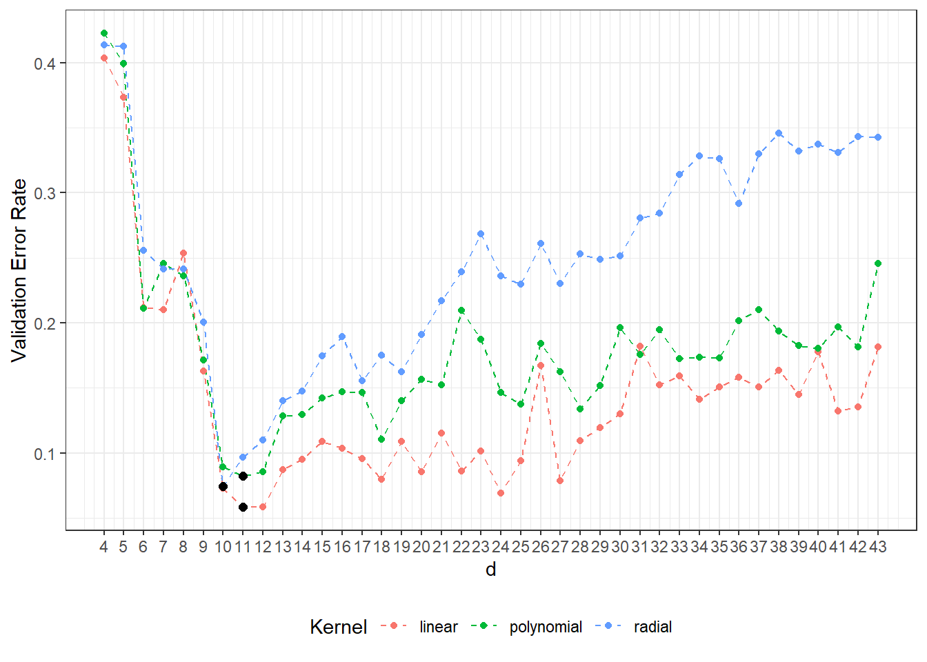

Dependence of validation error rate on subspace dimension $V_d$, for each of the three kernels considered in the SVM method. Optimal values of dimension $V_d$ for each kernel function are marked by black points.

Figure 1.24: Dependence of validation error rate on subspace dimension $V_d$, for each of the three kernels considered in the SVM method. Optimal values of dimension $V_d$ for each kernel function are marked by black points.

Now, we can train individual classifiers on all training data and evaluate their accuracy on test data. For each kernel function, we select the dimension of the subspace onto which we project based on the cross-validation results.

In the variable Projection, we store the matrix of orthogonal projection coefficients:

\[ \texttt{Projection} = \begin{pmatrix} \langle x_1, \Psi_1 \rangle & \langle x_2, \Psi_1 \rangle & \cdots & \langle x_n, \Psi_1 \rangle\\ \langle x_1, \Psi_2 \rangle & \langle x_2, \Psi_2 \rangle & \cdots & \langle x_n, \Psi_2 \rangle\\ \vdots & \vdots & \ddots & \vdots \\ \langle x_1, \Psi_d \rangle & \langle x_2, \Psi_d \rangle & \dots & \langle x_n, \Psi_d \rangle \end{pmatrix}_{d \times n}. \]

Code

# Prepare data table for storing results
Res <- data.frame(model = c('SVM linear - projection', 
                            'SVM poly - projection', 
                            'SVM rbf - projection'), 
                  Err.train = NA,
                  Err.test = NA)

# Iterate over kernels
for (kernel_number in 1:3) {
  kernel_type <- c('linear', 'polynomial', 'radial')[kernel_number]
  # basis object
  bbasis <- create.bspline.basis(rangeval = rangeval, 
                                 nbasis = d.opt[kernel_number])
  
  # projection of discrete data onto B-spline basis
  Projection <- project.basis(y = XX, # matrix of discrete data
                              argvals = t, # vector of arguments
                              basisobj = bbasis) # basis object
  
  # split into training and testing data
  XX.train <- subset(t(Projection), split == TRUE)
  XX.test <- subset(t(Projection), split == FALSE)
  
  data.projection.train <- as.data.frame(XX.train)
  data.projection.train$Y <- factor(Y.train)
  
  data.projection.test <- as.data.frame(XX.test)
  data.projection.test$Y <- factor(Y.test)
  
  # construct model
  clf.SVM.projection <- svm(Y ~ ., data = data.projection.train,
                            type = 'C-classification',
                            scale = TRUE,
                            coef0 = 1,
                            kernel = kernel_type)
  
  # training data accuracy
  predictions.train <- predict(clf.SVM.projection, newdata = data.projection.train)
  presnost.train <- table(Y.train, predictions.train) |>
    prop.table() |> diag() |> sum()
    
  # test data accuracy
  predictions.test <- predict(clf.SVM.projection, newdata = data.projection.test)
  presnost.test <- table(Y.test, predictions.test) |>
    prop.table() |> diag() |> sum()
  
  # store results
  Res[kernel_number, c(2, 3)] <- 1 - c(presnost.train, presnost.test)
}

The error rate of the SVM method applied to basis coefficients on the training data is 4.29% for the linear kernel, 3.57% for the polynomial kernel, and 5% for the Gaussian kernel. On the test data, the error rate is 10% for the linear kernel, 8.33% for the polynomial kernel, and 10% for the radial kernel.

Code

RESULTS <- rbind(RESULTS, Res)

1.3.7.6 RKHS + SVM

In this section, we will look at another way to utilize support vector methods for classifying functional data. This time, we will again apply the well-known principle of first expressing functional data as some finite-dimensional objects, and then applying the classic SVM method to these objects.

However, in this case, we will also use the SVM method for the representation of functional data using a certain finite-dimensional object. As the name suggests, this involves a combination of two concepts: the support vector method and a space known in English literature as Reproducing Kernel Hilbert Space (RKHS). The key concept for this space is the kernel.

Definition 1.1 (Kernel) A kernel is a function $K : \mathcal{X} \times \mathcal{X} \rightarrow \mathbb{R}$ such that for every pair $\boldsymbol{x}, \tilde{\boldsymbol{x}} \in \mathcal{X}$ it holds that \[ K(\boldsymbol{x}, \tilde{\boldsymbol{x}}) = \big\langle \boldsymbol{\phi}(\boldsymbol{x}), \boldsymbol{\phi}(\tilde{\boldsymbol{x}}) \big\rangle_{\mathcal{H}}, \] where $\boldsymbol{\phi} : \mathcal{X} \rightarrow \mathcal{H}$ is a mapping from the space $\mathcal{X}$ to the space $\mathcal{H}$.

For a function to be a kernel, it must satisfy certain conditions.

Lemma 1.1 Let $\mathcal{X}$ be a Hilbert space. Then a symmetric function $K : \mathcal{X} \times \mathcal{X} \rightarrow \mathbb{R}$ is a kernel if for all $k \geq 1, \boldsymbol{x}_1, \dots, \boldsymbol{x}_k \in \mathcal{X}$ and $c_1, \dots, c_k \in \mathbb{R}$, it holds that \[ \sum_{i, j = 1}^k c_i c_j K(\boldsymbol{x}_i, \boldsymbol{x}_j) \geq 0. \]

The property above is called positive semidefiniteness. The following statement also holds.

Theorem 1.1 A function $K: \mathcal{X} \times \mathcal{X} \rightarrow \mathbb{R}$ is a kernel if and only if there exists a Hilbert space $\mathcal{H}$ and a mapping $\boldsymbol{\phi} : \mathcal{X} \rightarrow \mathcal{H}$ such that \[ K(\boldsymbol{x}, \tilde{\boldsymbol{x}}) = \big\langle \boldsymbol{\phi}(\boldsymbol{x}), \boldsymbol{\phi}(\tilde{\boldsymbol{x}}) \big\rangle_{\mathcal{H}} \quad \forall \boldsymbol{x}, \tilde{\boldsymbol{x}} \in \mathcal{X}. \]

Now we are ready to introduce the concept of Reproducing Kernel Hilbert Space.

1.3.7.6.1 Reproducing Kernel Hilbert Space (RKHS)

Consider a Hilbert space $\mathcal{H}$ as a space of functions. Our goal is to define the space $\mathcal{H}$ and the mapping $\phi$ such that $\phi(x) \in \mathcal{H}, \ \forall x \in \mathcal{X}$. Let $\phi(x) = k_x$. We assign to each function $x \in \mathcal{X}$ the function $x \mapsto k_x \in \mathcal{H}, k_x := K(x, \cdot)$. Then $\phi: \mathcal{X} \rightarrow \mathbb{R}^{\mathcal{X}}$, so we can summarize it as

\[ x \in \mathcal{X} \mapsto \phi(x) = k_x = K(x, \cdot) \in \mathcal{H}, \]

The point (function) $x \in \mathcal{X}$ is mapped to the function $k_x: \mathcal{X} \rightarrow \mathbb{R}, k_x(y) = K(x, y)$.

Consider the set of all images $\{k_x | x \in \mathcal{X}\}$ and define the linear span of this set of vectors as

\[ \mathcal{G} := \text{span}\{k_x | x \in \mathcal{X}\} = \left\{\sum_{i = 1}^r \alpha_i K(x_i, \cdot) \ \Big|\ \alpha_i \in \mathbb{R}, r \in \mathbb{N}, x_i \in \mathcal{X}\right\}. \]

Then the inner product is given by

\[ \langle k_x, k_y \rangle = \langle K(x, \cdot), K(y, \cdot) \rangle = K(x, y),\quad x, y \in \mathcal{X} \]

and generally

\[ f, g \in \mathcal{G}, f = \sum_i \alpha_i K(x_i, \cdot), g = \sum_j \beta_j K(y_j, \cdot), \\ \langle f, g \rangle_{\mathcal{G}} = \Big\langle \sum_i \alpha_i K(x_i, \cdot), \sum_j \beta_j K(y_j, \cdot) \Big\rangle = \sum_i\sum_j \alpha_i \beta_j \langle K(x_i, \cdot), K(y_j, \cdot) \rangle = \sum_i\sum_j \alpha_i \beta_j K(x_i, y_j). \]

The space $\mathcal{H} := \overline{\mathcal{G}}$, which is the closure of the space $\mathcal{G}$, is called the Reproducing Kernel Hilbert Space (RKHS). A significant property of this space is

\[ K(x, y) = \Big\langle \phi(x), \phi(y) \Big\rangle_{\mathcal{H}}. \]

Note: The name Reproducing comes from the following fact. Let $f = \sum_i \alpha_i K(x_i, \cdot)$ be any function. Then

\[\begin{align*} \langle K(x, \cdot), f \rangle &= \langle K(x, \cdot), \sum_i \alpha_i K(x_i, \cdot) \rangle =\\ &= \sum_i \alpha_i \langle K(x, \cdot), K(x_i, \cdot) \rangle = \sum_i \alpha_i K(x_i, x) = \\ &= f(x) \end{align*}\]

Properties:

Let $\mathcal{H}$ be a Hilbert space of functions $g: \mathcal{X} \rightarrow \mathbb{R}$. Then $\mathcal{H}$ is an RKHS if and only if all evaluation functionals $\delta_x: \mathcal{H} \rightarrow \mathbb{R}, g \mapsto g(x)$ are continuous.
For a given kernel $K$, there exists exactly one RKHS (up to isometric isomorphism).
For a given RKHS, the kernel $K$ is uniquely determined.
Functions in RKHS are pointwise well-defined.
RKHS is generally an infinite-dimensional vector space, but in practice, we only work with its finite-dimensional subspace.

At the end of this section, let us state an important theorem.

Theorem 1.2 (The representer theorem) Let $K$ be a kernel and $\mathcal H$ be the corresponding RKHS with norm and inner product $\|\cdot\|_{\mathcal H}$ and $\langle \cdot, \cdot \rangle_{\mathcal H}$. Suppose we want to find a linear function $f: \mathcal H \rightarrow \mathbb R$ in the Hilbert space $\mathcal H$ defined by the kernel $K$. The function $f$ has the form $f(x) = \langle \omega, x \rangle_{\mathcal H}$ for some $\omega \in \mathcal H$. Consider the regularized minimization problem:

\[\begin{equation} \min_{\omega \in \mathcal H} R_n(\omega) + \lambda \Omega(\|\omega\|_{\mathcal H}), \tag{1.1} \end{equation}\] where $\Omega: [0, \infty) \rightarrow \mathbb R$ is a strictly monotonically increasing function (regularizer), and $R_n(\cdot)$ is the empirical loss (empirical risk) of the classifier with respect to the loss function $\ell$. Then the optimization problem (1.1) always has an optimal solution, which is of the form:

\[\begin{equation} \omega^* = \sum_{i = 1}^n \alpha_i K(x_i, \cdot), \tag{1.2} \end{equation}\] where $(x_i, y_i)_{i = 1, 2, \dots, n} \in \mathcal X \times \mathcal Y$ is a set of training values.

$\mathcal H$ is generally an infinite-dimensional space, but for a finite dataset of size $n$, $\mathcal H$ has dimension at most $n$. Furthermore, every $n$-dimensional subspace of a Hilbert space is isometric to $\mathbb R^n$, so we can assume that the mapping (feature map) maps into $\mathbb R^n$.

The kernel $K$ is universal if the RKHS $\mathcal H$ is a dense subset of $\mathcal C(\mathcal X)$ (the set of continuous functions). Moreover, the following facts hold:

Universal kernels are good for approximation.
The Gaussian kernel with a fixed value $\sigma$ is universal.
Universality is a necessary condition for consistency.

1.3.7.6.2 Classification Using RKHS

The basic idea is to project the original data onto a subspace of the RKHS, denoted as $\mathcal H_K$ (the index ${}_K$ refers to the fact that this space is defined by the kernel $K$). The goal is to transform a curve (the observed object, function) into a point in the RKHS. Let us denote the set of observed curves as $\{\hat c_1, \dots, \hat c_n\}$, where each curve $\hat c_l$ is defined by the data $\{(\boldsymbol x_i, \boldsymbol y_{il}) \in \mathcal X \times \mathcal Y\}_{i = 1}^m$, with $\mathcal X$ being the space of input variables and typically $\mathcal Y = \mathbb R$. Assume that for each function $\hat c_l$, there exists a continuous function $c_l:\mathcal X \rightarrow \mathcal Y$ such that $\mathbb E[y_l|\boldsymbol x] = c_l(\boldsymbol x)$. We also assume that $\boldsymbol x_i$ are common to all curves.

Muñoz and González in their paper¹ propose the following procedure. The curve $c_l^*$ can be expressed as

\[ c_l^*(\boldsymbol x) = \sum_{i = 1}^m \alpha_{il} K(\boldsymbol x_i, \boldsymbol x), \quad \forall \boldsymbol x \in \mathcal X, \]

where $\alpha_{il} \in \mathbb R$. These coefficients can be obtained in practice by solving the optimization problem

\[ \text{argmin}_{c \in \mathcal H_K} \frac{1}{m} \sum_{i = 1}^m \big[|c(\boldsymbol x_i) - y_i| - \varepsilon\big]_+ + \gamma \|c\|_{K}^2, \quad \gamma > 0, \varepsilon \geq 0, \]

specifically, for example, using the SVM method. Due to the well-known property of this method, many coefficients will be $\alpha_{il} = 0$. By minimizing the above expression, we obtain functions $c_1^*, \dots, c_n^*$ corresponding to the original curves $\hat c_1, \dots, \hat c_n$. Thus, the SVM method provides a meaningful representation of the original curves using the coefficient vector $\boldsymbol \alpha_l = (\alpha_{1l}, \dots, \alpha_{ml})^\top$ for $\hat c_l$. However, this representation is very unstable, as even a small change in the original values can lead to a change in the set of support vectors for the given function, resulting in a significant change in the entire representation of this curve (the representation is not continuous in the input values). Therefore, we define a new representation of the original curves that will not suffer from this drawback.

Theorem 1.3 (Muñoz-González) Let $c$ be a function whose observed version is $\hat c = \{(\boldsymbol x_i, y_{i}) \in \mathcal X \times \mathcal Y\}_{i = 1}^m$, and let $K$ be a kernel with eigenfunctions $\{\phi_1, \dots, \phi_d, \dots\}$ (basis of $\mathcal H_K$). Then the function $c^*(\boldsymbol x)$ can be expressed in the form \[\begin{equation*} c^*(\boldsymbol x) = \sum_{j = 1}^d \lambda_j^* \phi_j(\boldsymbol x), \end{equation*}\] where $\lambda_j^*$ are the weights of the projection of $c^*(\boldsymbol x)$ onto the space of functions generated by the eigenfunctions of the kernel $K$, and $d$ is the dimension of the space $\mathcal H$. In practice, when we only have a finite number of observations, $\lambda_j^*$ can be estimated using \[\begin{equation*} \hat\lambda_j^* = \hat\lambda_j \sum_{i = 1}^m \alpha_i\hat\phi_{ji}, \quad j = 1, 2, \dots, \hat d, \end{equation*}\] where $\hat\lambda_j$ is the $j$-th eigenvalue corresponding to the $j$-th eigenvector $\hat\phi_j$ of the matrix $K_S = \big(K(\boldsymbol x_i, \boldsymbol x_j)\big)_{i, j = 1}^m$, $\hat d = \text{rank}(K_S)$, and $\alpha_i$ are the solutions to the optimization problem.

1.3.7.6.3 Implementation of the Method in `R`

From the last part of Theorem 1.3, it follows how we should compute the representations of the curves in practice. We will work with discretized data after smoothing the curves. First, we define the kernel for the RKHS space. We will use the Gaussian kernel with parameter $\gamma$. The value of this hyperparameter significantly affects the behavior and thus the success of the method, so we must pay special attention to its selection (we choose it using cross-validation).

1.3.7.6.3.1 Gaussian Kernel

Code

# Remove the last column, which contains the Y values
data.RKHS <- grid.data[, -dim(grid.data)[2]] |> t()
# Add the test data as well
data.RKHS <- cbind(data.RKHS, grid.data.test[, -dim(grid.data.test)[2]] |> t())

# Kernel and kernel matrix ... Gaussian with parameter gamma
Gauss.kernel <- function(x, y, gamma) {
  return(exp(-gamma * norm(c(x - y) |> t(), type = 'F')))
}

Kernel.RKHS <- function(x, gamma) {
  K <- matrix(NA, ncol = length(x), nrow = length(x))
  for(i in 1:nrow(K)) {
    for(j in 1:ncol(K)) {
      K[i, j] <- Gauss.kernel(x = x[i], y = x[j], gamma = gamma)
    }
  }
  return(K)
}

Now let’s calculate the matrix $K_S$ and its eigenvalues and corresponding eigenvectors.

Code

# Calculate the matrix K
gamma <- 0.1 # Fixed value of gamma; we will determine the optimal value using CV
K <- Kernel.RKHS(t.seq, gamma = gamma)

# Determine eigenvalues and eigenvectors
Eig <- eigen(K)
eig.vals <- Eig$values
eig.vectors <- Eig$vectors

To calculate the coefficients in the representation of the curves, i.e., the vectors $\hat{\boldsymbol \lambda}_l^* = \left( \hat\lambda_{1l}^*, \dots, \hat\lambda_{\hat d l}^*\right)^\top, l = 1, 2, \dots, n$, we also need the coefficients from the SVM. Unlike the classification problem, we are now solving a regression problem, as we are trying to express our observed curves in some basis (chosen by us via the kernel $K$). Therefore, we will use the Support Vector Regression method, from which we will subsequently obtain the coefficients $\alpha_{il}$.

Code

# Determine coefficients alpha from SVM
alpha.RKHS <- matrix(0, nrow = dim(data.RKHS)[1],
                     ncol = dim(data.RKHS)[2]) # Empty object

# Model
for(i in 1:dim(data.RKHS)[2]) {
  df.svm <- data.frame(x = t.seq,
                       y = data.RKHS[, i])
  svm.RKHS <- svm(y ~ x, data = df.svm, 
                  kernel = 'radial',
                  type = 'eps-regression',
                  epsilon = 0.1,
                  gamma = gamma)
  # Determine alpha
  alpha.RKHS[svm.RKHS$index, i] <- svm.RKHS$coefs # Replace zeros with coefficients
}

Now we can calculate the representations of the individual curves. First, let’s choose $\hat d$ as the entire dimension, i.e., $\hat d = m ={}$ 101, and then we will determine the optimal $\hat d$ using cross-validation.

Code

# d
d.RKHS <- dim(alpha.RKHS)[1]

# Determine the lambda vector
Lambda.RKHS <- matrix(NA, 
                      ncol = dim(data.RKHS)[2], 
                      nrow = d.RKHS) # Create an empty object

# Calculate the representation
for(l in 1:dim(data.RKHS)[2]) {
  Lambda.RKHS[, l] <- (t(eig.vectors[, 1:d.RKHS]) %*% alpha.RKHS[, l]) * eig.vals[1:d.RKHS]
}

Now we have the vectors $\hat{\boldsymbol \lambda}_l^*, l = 1, 2, \dots, n$ stored in the columns of the matrix Lambda.RKHS for each curve. We will now use these vectors as the representation of the given curves and classify the data according to this discretization.

Code

# Split into training and testing data
XX.train <- Lambda.RKHS[, 1:dim(grid.data)[1]]
XX.test <- Lambda.RKHS[, (dim(grid.data)[1] + 1):dim(Lambda.RKHS)[2]]

# Prepare a data table to store results
Res <- data.frame(model = c('SVM linear - RKHS', 
                            'SVM poly - RKHS', 
                            'SVM rbf - RKHS'), 
                  Err.train = NA,
                  Err.test = NA)

# Loop through each kernel
for (kernel_number in 1:3) {
  kernel_type <- c('linear', 'polynomial', 'radial')[kernel_number]

  data.RKHS.train <- as.data.frame(t(XX.train))
  data.RKHS.train$Y <- factor(Y.train)
  
  data.RKHS.test <- as.data.frame(t(XX.test))
  data.RKHS.test$Y <- factor(Y.test)
  
  # Build models
  clf.SVM.RKHS <- svm(Y ~ ., data = data.RKHS.train,
                      type = 'C-classification',
                      scale = TRUE,
                      coef0 = 1,
                      kernel = kernel_type)
  
  # Accuracy on training data
  predictions.train <- predict(clf.SVM.RKHS, newdata = data.RKHS.train)
  accuracy.train <- table(Y.train, predictions.train) |>
    prop.table() |> diag() |> sum()
    
  # Accuracy on testing data
  predictions.test <- predict(clf.SVM.RKHS, newdata = data.RKHS.test)
  accuracy.test <- table(Y.test, predictions.test) |>
    prop.table() |> diag() |> sum()
  
  # Save results
  Res[kernel_number, c(2, 3)] <- 1 - c(accuracy.train, accuracy.test)
}

Table 1.1: Summary results of the SVM method combined with RKHS on simulated data. $\widehat{Err}_{train}$ indicates the estimate of training error and $\widehat{Err}_{test}$ the testing error.
Model	$\widehat{Err}_{train}\quad\quad\quad\quad\quad$	$\widehat{Err}_{test}\quad\quad\quad\quad\quad$
SVM linear - RKHS	0.1000	0.3833
SVM poly - RKHS	0.0286	0.3000
SVM rbf - RKHS	0.0786	0.2667

We see that the model performs very well on the training data for all three kernels, while its performance on the testing data is not good at all. It is clear that overfitting has occurred; therefore, we will use cross-validation to determine the optimal values of $\gamma$ and $d$.

Code

# Split the training data into k parts
folds <- createMultiFolds(1:sum(split), k = k_cv, time = 1)
# Remove the last column, which contains the Y values
data.RKHS <- grid.data[, -dim(grid.data)[2]] |> t()

# Hyperparameter values to iterate over
dimensions <- 3:40 # Reasonable range of values for d
gamma.cv <- 10^seq(-1, 2, length = 15)

# List with three components ... array for individual kernels -> linear, poly, radial
# Empty matrix to insert individual results
# Columns will contain accuracy values for given
# Rows will contain values for given gamma and layers will correspond to folds
dim.names <- list(gamma = paste0('gamma:', round(gamma.cv, 3)),
                  d = paste0('d:', dimensions),
                  CV = paste0('cv:', 1:k_cv))

CV.results <- list(
  SVM.l = array(NA, dim = c(length(gamma.cv), length(dimensions), k_cv),
                dimnames = dim.names),
  SVM.p = array(NA, dim = c(length(gamma.cv), length(dimensions), k_cv),
                dimnames = dim.names),
  SVM.r = array(NA, dim = c(length(gamma.cv), length(dimensions), k_cv),
                dimnames = dim.names))

Code

# Cross-validation
for (gamma in gamma.cv) {
  K <- Kernel.RKHS(t.seq, gamma = gamma)
  Eig <- eigen(K)
  eig.vals <- Eig$values
  eig.vectors <- Eig$vectors
  alpha.RKHS <- matrix(0, nrow = dim(data.RKHS)[1], ncol = dim(data.RKHS)[2]) 
  
  # Model
  for(i in 1:dim(data.RKHS)[2]) {
    df.svm <- data.frame(x = t.seq,
                         y = data.RKHS[, i])
    svm.RKHS <- svm(y ~ x, data = df.svm, 
                    kernel = 'radial',
                    type = 'eps-regression',
                    epsilon = 0.1,
                    gamma = gamma)
    alpha.RKHS[svm.RKHS$index, i] <- svm.RKHS$coefs 
  }
  
  # Iterate over dimensions
  for(d.RKHS in dimensions) {
    Lambda.RKHS <- matrix(NA, 
                          ncol = dim(data.RKHS)[2], 
                          nrow = d.RKHS) 
    # Calculate representation
    for(l in 1:dim(data.RKHS)[2]) {
      Lambda.RKHS[, l] <- (t(eig.vectors[, 1:d.RKHS]) %*% 
                             alpha.RKHS[, l]) * eig.vals[1:d.RKHS]
    }
    # Iterate over folds
    for (index_cv in 1:k_cv) {
      # Define testing and training parts for CV
      fold <- folds[[index_cv]]
      # Split into training and validation data
      XX.train <- Lambda.RKHS[, fold]
      XX.test <- Lambda.RKHS[, !(1:dim(Lambda.RKHS)[2] %in% fold)]
      # Prepare a data table to store results
      Res <- data.frame(model = c('SVM linear - RKHS', 
                                  'SVM poly - RKHS', 
                                  'SVM rbf - RKHS'), 
                        Err.test = NA)
      # Iterate over individual kernels
      for (kernel_number in 1:3) {
        kernel_type <- c('linear', 'polynomial', 'radial')[kernel_number]
      
        data.RKHS.train <- as.data.frame(t(XX.train))
        data.RKHS.train$Y <- factor(Y.train[fold])
        
        data.RKHS.test <- as.data.frame(t(XX.test))
        data.RKHS.test$Y <- factor(Y.train[!(1:dim(Lambda.RKHS)[2] %in% fold)])
        
        # Build models
        clf.SVM.RKHS <- svm(Y ~ ., data = data.RKHS.train,
                            type = 'C-classification',
                            scale = TRUE,
                            coef0 = 1,
                            kernel = kernel_type)
        
        # Accuracy on validation data
        predictions.test <- predict(clf.SVM.RKHS, newdata = data.RKHS.test)
        accuracy.test <- table(data.RKHS.test$Y, predictions.test) |>
          prop.table() |> diag() |> sum()
        
        # Save results
        Res[kernel_number, 2] <- 1 - accuracy.test
      }
      # Insert accuracies for the given d, gamma, and fold
      CV.results$SVM.l[paste0('gamma:', round(gamma, 3)), 
                       d.RKHS - min(dimensions) + 1, 
                       index_cv] <- Res[1, 2]
      CV.results$SVM.p[paste0('gamma:', round(gamma, 3)), 
                       d.RKHS - min(dimensions) + 1, 
                       index_cv] <- Res[2, 2]
      CV.results$SVM.r[paste0('gamma:', round(gamma, 3)), 
                       d.RKHS - min(dimensions) + 1, 
                       index_cv] <- Res[3, 2]
    }
  }
}

Code

# Calculate average accuracies for each d across folds
for (n_method in 1:length(CV.results)) {
  CV.results[[n_method]] <- apply(CV.results[[n_method]], c(1, 2), mean)
}

gamma.opt <- c(which.min(CV.results$SVM.l) %% length(gamma.cv), 
               which.min(CV.results$SVM.p) %% length(gamma.cv), 
               which.min(CV.results$SVM.r) %% length(gamma.cv))
gamma.opt[gamma.opt == 0] <- length(gamma.cv)
gamma.opt <- gamma.cv[gamma.opt]

d.opt <- c(which.min(t(CV.results$SVM.l)) %% length(dimensions), 
           which.min(t(CV.results$SVM.p)) %% length(dimensions), 
           which.min(t(CV.results$SVM.r)) %% length(dimensions))
d.opt[d.opt == 0] <- length(dimensions)
d.opt <- dimensions[d.opt]

err.opt.cv <- c(min(CV.results$SVM.l), 
                     min(CV.results$SVM.p),
                     min(CV.results$SVM.r))
df.RKHS.res <- data.frame(d = d.opt, gamma = gamma.opt, CV = err.opt.cv,
           Kernel = c('linear', 'polynomial', 'radial') |> factor(),
           row.names = c('linear', 'poly', 'radial'))

Table 1.2: Summary results of cross-validation for the SVM method combined with RKHS on simulated data. $\widehat{Err}_{train}$ indicates the estimate of training error and $\widehat{Err}_{test}$ the testing error.
	$\quad\quad\quad\quad\quad d$	$\quad\quad\quad\quad\quad\gamma$	$\widehat{Err}_{cross\_validace}$	Model
linear	10	8.4834	0.0728	linear
poly	17	8.4834	0.0870	polynomial
radial	38	0.4394	0.1054	radial

We see that the best parameter values are $d={}$ 10 and $\gamma={}$ 8.4834 for the linear kernel, with the error calculated using 10-fold CV being 0.0728. Similarly, $d={}$ 17 and $\gamma={}$ 8.4834 for the polynomial kernel, with an error of 0.087, and $d={}$ 38 and $\gamma={}$ 0.4394 for the radial kernel, yielding an error of 0.1054.

For interest, let’s plot the validation error as a function of dimension $d$ and the hyperparameter $\gamma$.

Code

CV.results.plot <- data.frame(d = rep(dimensions |> rep(3), each = length(gamma.cv)), 
                              gamma = rep(gamma.cv, length(dimensions)) |> rep(3),
                               CV = c(c(CV.results$SVM.l), 
                                      c(CV.results$SVM.p), 
                                      c(CV.results$SVM.r)),
                               Kernel = rep(c('linear', 'polynomial', 'radial'), 
                                            each = length(dimensions) * 
                                              length(gamma.cv)) |> factor())
CV.results.plot |> 
  ggplot(aes(x = d, y = gamma, z = CV)) + 
  geom_contour_filled() +
  scale_y_continuous(trans='log10') +
  facet_wrap(~Kernel) +
  theme_bw() + 
  labs(x = expression(d),
       y = expression(gamma)) + 
  scale_fill_brewer(palette = "Spectral") + 
  geom_point(data = df.RKHS.res, aes(x = d, y = gamma),
             size = 5, pch = '+')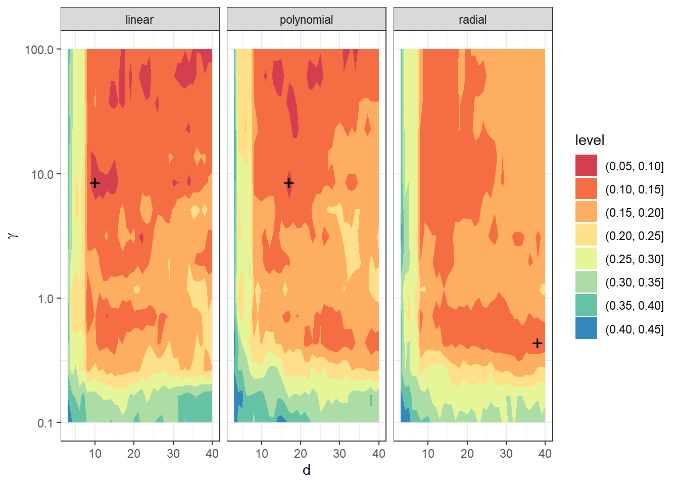

$Dependence of validation error on the choice of hyperparameters $d$ and $\gamma$, separately for all three considered kernels in the SVM method.$

Figure 1.25: Dependence of validation error on the choice of hyperparameters $d$ and $\gamma$, separately for all three considered kernels in the SVM method.

In the above plots, we can see how the validation error changed with the values of hyperparameters $d$ and $\gamma$. Notably, in all three plots for the individual kernels, significant horizontal patterns are visible. From this, we can draw a significant theoretical and practical conclusion: the considered classification method (projection onto RKHS using SVM + SVM classification) is robust to the choice of the hyperparameter $d$ (i.e., a small change in this parameter’s value does not lead to a significant deterioration in validation error), while we must be very cautious with the choice of the hyperparameter $\gamma$ (even a small change in its value can lead to a large change in validation error). This behavior is most apparent with the Gaussian kernel.

Since we have already found the optimal values of the hyperparameters, we can construct the final models and determine their classification success on the test data.

Code

# Remove the last column, which contains the Y values
data.RKHS <- grid.data[, -dim(grid.data)[2]] |> t()
# Add the test data as well
data.RKHS <- cbind(data.RKHS, grid.data.test[, -dim(grid.data.test)[2]] |> t())

Code

# Prepare a data table to store results
Res <- data.frame(model = c('SVM linear - RKHS - radial', 
                            'SVM poly - RKHS - radial', 
                            'SVM rbf - RKHS - radial'), 
                  Err.train = NA,
                  Err.test = NA)

# Loop through the individual kernels
for (kernel_number in 1:3) {
  # Calculate the K matrix
  gamma <- gamma.opt[kernel_number] # gamma value from CV
  K <- Kernel.RKHS(t.seq, gamma = gamma)
  
  # Determine eigenvalues and eigenvectors
  Eig <- eigen(K)
  eig.vals <- Eig$values
  eig.vectors <- Eig$vectors
  # Determine the coefficients alpha from SVM
  alpha.RKHS <- matrix(0, nrow = dim(data.RKHS)[1],
                       ncol = dim(data.RKHS)[2]) # empty object
  
  # Model
  for(i in 1:dim(data.RKHS)[2]) {
    df.svm <- data.frame(x = t.seq,
                         y = data.RKHS[, i])
    svm.RKHS <- svm(y ~ x, data = df.svm, 
                    kernel = 'radial',
                    type = 'eps-regression',
                    epsilon = 0.1,
                    gamma = gamma)
    # Determine alpha
    alpha.RKHS[svm.RKHS$index, i] <- svm.RKHS$coefs # replace zeros with coefficients
  }
  # d
  d.RKHS <- d.opt[kernel_number]
  
  # Determine the lambda vector
  Lambda.RKHS <- matrix(NA, 
                        ncol = dim(data.RKHS)[2], 
                        nrow = d.RKHS) # create an empty object
  
  # Compute the representation
  for(l in 1:dim(data.RKHS)[2]) {
    Lambda.RKHS[, l] <- (t(eig.vectors[, 1:d.RKHS]) %*% alpha.RKHS[, l]) * eig.vals[1:d.RKHS]
  }
  
  # Split into training and test data
  XX.train <- Lambda.RKHS[, 1:dim(grid.data)[1]]
  XX.test <- Lambda.RKHS[, (dim(grid.data)[1] + 1):dim(Lambda.RKHS)[2]]

  kernel_type <- c('linear', 'polynomial', 'radial')[kernel_number]

  data.RKHS.train <- as.data.frame(t(XX.train))
  data.RKHS.train$Y <- factor(Y.train)
  
  data.RKHS.test <- as.data.frame(t(XX.test))
  data.RKHS.test$Y <- factor(Y.test)
  
  # Model construction
  clf.SVM.RKHS <- svm(Y ~ ., data = data.RKHS.train,
                      type = 'C-classification',
                      scale = TRUE,
                      coef0 = 1,
                      kernel = kernel_type)
  
  # Accuracy on training data
  predictions.train <- predict(clf.SVM.RKHS, newdata = data.RKHS.train)
  presnost.train <- table(Y.train, predictions.train) |>
    prop.table() |> diag() |> sum()
    
  # Accuracy on test data
  predictions.test <- predict(clf.SVM.RKHS, newdata = data.RKHS.test)
  presnost.test <- table(Y.test, predictions.test) |>
    prop.table() |> diag() |> sum()
  
  # Save results
  Res[kernel_number, c(2, 3)] <- 1 - c(presnost.train, presnost.test)
}

Table 1.3: Summary results of the SVM method combined with RKHS on simulated data. $\widehat{Err}_{train}$ denotes the estimated training error and $\widehat{Err}_{test}$ the test error.
Model	$\widehat{Err}_{train}\quad\quad\quad\quad\quad$	$\widehat{Err}_{test}\quad\quad\quad\quad\quad$
SVM linear - RKHS - radial	0.0500	0.1333
SVM poly - RKHS - radial	0.0143	0.2000
SVM rbf - RKHS - radial	0.0143	0.1333

The error rate of the SVM method combined with the projection onto the Reproducing Kernel Hilbert Space is thus equal to 5 % for the linear kernel, 1.43 % for the polynomial kernel, and 1.43 % for the Gaussian kernel on the training data. For the test data, the error rate of the method is 13.33 % for the linear kernel, 20 % for the polynomial kernel, and 13.33 % for the radial kernel.

Code

RESULTS <- rbind(RESULTS, Res)

1.3.7.6.3.2 Polynomial Kernel

Code

# Remove the last column, which contains the values of Y
data.RKHS <- grid.data[, -dim(grid.data)[2]] |> t()
# Add test data as well
data.RKHS <- cbind(data.RKHS, grid.data.test[, -dim(grid.data.test)[2]] |> t())

# Kernel and kernel matrix... polynomial with parameter p
Poly.kernel <- function(x, y, p) {
  return((1 + x * y)^p)
}

Kernel.RKHS <- function(x, p) {
  K <- matrix(NA, ncol = length(x), nrow = length(x))
  for(i in 1:nrow(K)) {
    for(j in 1:ncol(K)) {
      K[i, j] <- Poly.kernel(x = x[i], y = x[j], p)
    }
  }
  return(K)
}

Code

# Split training data into k parts
folds <- createMultiFolds(1:sum(split), k = k_cv, time = 1)
# Remove the last column, which contains the values of Y
data.RKHS <- grid.data[, -dim(grid.data)[2]] |> t()

# Values of hyperparameters to iterate over
dimensions <- 3:40 # reasonable range of values d
poly.cv <- 2:5

# List with three components... array for individual kernels -> linear, poly, radial
# Empty matrix to store individual results
# Columns will have accuracy values for the given
# Rows will have values for the given p, and layers correspond to folds
dim.names <- list(p = paste0('p:', poly.cv),
                  d = paste0('d:', dimensions),
                  CV = paste0('cv:', 1:k_cv))

CV.results <- list(
  SVM.l = array(NA, dim = c(length(poly.cv), length(dimensions), k_cv),
                dimnames = dim.names),
  SVM.p = array(NA, dim = c(length(poly.cv), length(dimensions), k_cv),
                dimnames = dim.names),
  SVM.r = array(NA, dim = c(length(poly.cv), length(dimensions), k_cv),
                dimnames = dim.names))

Code

# Cross-validation
for (p in poly.cv) {
  K <- Kernel.RKHS(t.seq, p = p)
  Eig <- eigen(K)
  eig.vals <- Eig$values
  eig.vectors <- Eig$vectors
  alpha.RKHS <- matrix(0, nrow = dim(data.RKHS)[1], ncol = dim(data.RKHS)[2]) 
  
  # Model
  for(i in 1:dim(data.RKHS)[2]) {
    df.svm <- data.frame(x = t.seq,
                         y = data.RKHS[, i])
    svm.RKHS <- svm(y ~ x, data = df.svm, 
                    kernel = 'polynomial',
                    type = 'eps-regression',
                    epsilon = 0.1,
                    coef0 = 1,
                    degree = p)
    alpha.RKHS[svm.RKHS$index, i] <- svm.RKHS$coefs 
  }
  
  # Iterate over dimensions
  for(d.RKHS in dimensions) {
    Lambda.RKHS <- matrix(NA, 
                          ncol = dim(data.RKHS)[2], 
                          nrow = d.RKHS) 
    # Compute representation
    for(l in 1:dim(data.RKHS)[2]) {
      Lambda.RKHS[, l] <- (t(eig.vectors[, 1:d.RKHS]) %*% 
                             alpha.RKHS[, l]) * eig.vals[1:d.RKHS]
    }
    # Iterate over folds
    for (index_cv in 1:k_cv) {
      # Define test and training parts for CV
      fold <- folds[[index_cv]]
      # Split into training and validation data
      XX.train <- Lambda.RKHS[, fold]
      XX.test <- Lambda.RKHS[, !(1:dim(Lambda.RKHS)[2] %in% fold)]
      # Prepare a data table to store results
      Res <- data.frame(model = c('SVM linear - RKHS', 
                                  'SVM poly - RKHS', 
                                  'SVM rbf - RKHS'), 
                        Err.test = NA)
      # Iterate over individual kernels
      for (kernel_number in 1:3) {
        kernel_type <- c('linear', 'polynomial', 'radial')[kernel_number]
      
        data.RKHS.train <- as.data.frame(t(XX.train))
        data.RKHS.train$Y <- factor(Y.train[fold])
        
        data.RKHS.test <- as.data.frame(t(XX.test))
        data.RKHS.test$Y <- factor(Y.train[!(1:dim(Lambda.RKHS)[2] %in% fold)])
        
        # Construct models
        clf.SVM.RKHS <- svm(Y ~ ., data = data.RKHS.train,
                            type = 'C-classification',
                            scale = TRUE,
                            coef0 = 1,
                            kernel = kernel_type)
        
        # Accuracy on validation data
        predictions.test <- predict(clf.SVM.RKHS, newdata = data.RKHS.test)
        presnost.test <- table(data.RKHS.test$Y, predictions.test) |>
          prop.table() |> diag() |> sum()
        
        # Save results
        Res[kernel_number, 2] <- 1 - presnost.test
      }
      # Store accuracies for the given d, gamma, and fold
      CV.results$SVM.l[paste0('p:', p), 
                       d.RKHS - min(dimensions) + 1, 
                       index_cv] <- Res[1, 2]
      CV.results$SVM.p[paste0('p:', p), 
                       d.RKHS - min(dimensions) + 1, 
                       index_cv] <- Res[2, 2]
      CV.results$SVM.r[paste0('p:', p), 
                       d.RKHS - min(dimensions) + 1, 
                       index_cv] <- Res[3, 2]
    }
  }
}

Code

# Calculate the average accuracy for each d across folds
for (n_method in 1:length(CV.results)) {
  CV.results[[n_method]] <- apply(CV.results[[n_method]], c(1, 2), mean)
}

poly.opt <- c(which.min(CV.results$SVM.l) %% length(poly.cv), 
               which.min(CV.results$SVM.p) %% length(poly.cv), 
               which.min(CV.results$SVM.r) %% length(poly.cv))
poly.opt[poly.opt == 0] <- length(poly.cv)
poly.opt <- poly.cv[poly.opt]

d.opt <- c(which.min(t(CV.results$SVM.l)) %% length(dimensions), 
           which.min(t(CV.results$SVM.p)) %% length(dimensions), 
           which.min(t(CV.results$SVM.r)) %% length(dimensions))
d.opt[d.opt == 0] <- length(dimensions)
d.opt <- dimensions[d.opt]

err.opt.cv <- c(min(CV.results$SVM.l), 
                 min(CV.results$SVM.p),
                 min(CV.results$SVM.r))
df.RKHS.res <- data.frame(d = d.opt, p = poly.opt, CV = err.opt.cv,
           Kernel = c('linear', 'polynomial', 'radial') |> factor(),
           row.names = c('linear', 'poly', 'radial'))

Table 1.4: Summary results of cross-validation for the SVM method combined with RKHS on simulated data. $\widehat{Err}_{train}$ denotes the estimate of training error and $\widehat{Err}_{test}$ the testing error.
	$\quad\quad\quad\quad\quad d$	$\quad\quad\quad\quad\quad p$	$\widehat{Err}_{cross\_validation}$	Model
linear	17	4	0.1412	linear
poly	10	4	0.1429	polynomial
radial	38	4	0.1550	radial

We see that the best values for the parameter $d={}$ 17 and $p={}$ 4 are for the linear kernel, with an error value computed using 10-fold CV of 0.1412. The values $d={}$ 10 and $p={}$ 4 are for the polynomial kernel, with an error value computed using 10-fold CV of 0.1429, and $d={}$ 38 and $p={}$ 4 are for the radial kernel, with an error value of 0.155.

Since we have found the optimal values of the hyperparameters, we can construct the final models and determine their classification success on the test data.

Code

# Remove the last column, which contains the values of Y
data.RKHS <- grid.data[, -dim(grid.data)[2]] |> t()
# Add the test data as well
data.RKHS <- cbind(data.RKHS, grid.data.test[, -dim(grid.data.test)[2]] |> t())

Code

# Prepare a data table to store results
Res <- data.frame(model = c('SVM linear - RKHS - poly', 
                            'SVM poly - RKHS - poly', 
                            'SVM rbf - RKHS - poly'), 
                  Err.train = NA,
                  Err.test = NA)

# Loop through individual kernels
for (kernel_number in 1:3) {
  # Calculate matrix K
  p <- poly.opt[kernel_number] # value of gamma from CV
  K <- Kernel.RKHS(t.seq, p = p)
  
  # Determine eigenvalues and eigenvectors
  Eig <- eigen(K)
  eig.vals <- Eig$values
  eig.vectors <- Eig$vectors
  # Determine alpha coefficients from SVM
  alpha.RKHS <- matrix(0, nrow = dim(data.RKHS)[1],
                       ncol = dim(data.RKHS)[2]) # empty object
  
  # Model
  for(i in 1:dim(data.RKHS)[2]) {
    df.svm <- data.frame(x = t.seq,
                         y = data.RKHS[, i])
    svm.RKHS <- svm(y ~ x, data = df.svm, 
                    kernel = 'polynomial',
                    type = 'eps-regression',
                    epsilon = 0.1,
                    coef0 = 1,
                    degree = p)
    # Determine alpha
    alpha.RKHS[svm.RKHS$index, i] <- svm.RKHS$coefs # replace zeros with coefficients
  }
  # d
  d.RKHS <- d.opt[kernel_number]
  
  # Determine the lambda vector
  Lambda.RKHS <- matrix(NA, 
                        ncol = dim(data.RKHS)[2], 
                        nrow = d.RKHS) # create an empty object
  
  # Compute representation
  for(l in 1:dim(data.RKHS)[2]) {
    Lambda.RKHS[, l] <- (t(eig.vectors[, 1:d.RKHS]) %*% alpha.RKHS[, l]) * eig.vals[1:d.RKHS]
  }
  
  # Split into training and test data
  XX.train <- Lambda.RKHS[, 1:dim(grid.data)[1]]
  XX.test <- Lambda.RKHS[, (dim(grid.data)[1] + 1):dim(Lambda.RKHS)[2]]

  kernel_type <- c('linear', 'polynomial', 'radial')[kernel_number]

  data.RKHS.train <- as.data.frame(t(XX.train))
  data.RKHS.train$Y <- factor(Y.train)
  
  data.RKHS.test <- as.data.frame(t(XX.test))
  data.RKHS.test$Y <- factor(Y.test)
  
  # Model construction
  clf.SVM.RKHS <- svm(Y ~ ., data = data.RKHS.train,
                      type = 'C-classification',
                      scale = TRUE,
                      coef0 = 1,
                      kernel = kernel_type)
  
  # Accuracy on training data
  predictions.train <- predict(clf.SVM.RKHS, newdata = data.RKHS.train)
  accuracy.train <- table(Y.train, predictions.train) |>
    prop.table() |> diag() |> sum()
    
  # Accuracy on test data
  predictions.test <- predict(clf.SVM.RKHS, newdata = data.RKHS.test)
  accuracy.test <- table(Y.test, predictions.test) |>
    prop.table() |> diag() |> sum()
  
  # Save results
  Res[kernel_number, c(2, 3)] <- 1 - c(accuracy.train, accuracy.test)
}

Table 1.5: Summary results of the SVM method combined with RKHS on simulated data. $\widehat{Err}_{train}$ denotes the estimate of training error and $\widehat{Err}_{test}$ the testing error.
Model	$\widehat{Err}_{train}\quad\quad\quad\quad\quad$	$\widehat{Err}_{test}\quad\quad\quad\quad\quad$
SVM linear - RKHS - poly	0.1071	0.2167
SVM poly - RKHS - poly	0.0643	0.2000
SVM rbf - RKHS - poly	0.1000	0.2333

The error rate of the SVM method combined with projection onto the Reproducing Kernel Hilbert Space is thus 10.71 % for the linear kernel, 6.43 % for the polynomial kernel, and 10 % for the Gaussian kernel. On the test data, the error rate of the method is 21.67 % for the linear kernel, 20 % for the polynomial kernel, and 23.33 % for the radial kernel.

Code

RESULTS <- rbind(RESULTS, Res)

1.3.7.6.3.3 Linear Kernel

Code

# Remove the last column containing Y values
data.RKHS <- grid.data[, -dim(grid.data)[2]] |> t()
# Add the test data as well
data.RKHS <- cbind(data.RKHS, grid.data.test[, -dim(grid.data.test)[2]] |> t())

# Kernel and kernel matrix ... polynomial with parameter p
Linear.kernel <- function(x, y) {
  return(x * y)
}

Kernel.RKHS <- function(x) {
  K <- matrix(NA, ncol = length(x), nrow = length(x))
  for(i in 1:nrow(K)) {
    for(j in 1:ncol(K)) {
      K[i, j] <- Linear.kernel(x = x[i], y = x[j])
    }
  }
  return(K)
}

Code

# Split training data into k parts
folds <- createMultiFolds(1:sum(split), k = k_cv, time = 1)
# Remove the last column containing Y values
data.RKHS <- grid.data[, -dim(grid.data)[2]] |> t()

# Hyperparameter values to iterate through
dimensions <- 3:40 # reasonable range of values for d

# List with three components ... array for individual kernels -> linear, poly, radial
# Empty matrix to store individual results
# Columns will hold accuracy values for given d
# Rows will hold values for layers corresponding to folds
dim.names <- list(d = paste0('d:', dimensions),
                  CV = paste0('cv:', 1:k_cv))

CV.results <- list(
  SVM.l = array(NA, dim = c(length(dimensions), k_cv),
                dimnames = dim.names),
  SVM.p = array(NA, dim = c(length(dimensions), k_cv),
                dimnames = dim.names),
  SVM.r = array(NA, dim = c(length(dimensions), k_cv),
                dimnames = dim.names))

Code

# Cross-validation itself
K <- Kernel.RKHS(t.seq)
Eig <- eigen(K)
eig.vals <- Eig$values
eig.vectors <- Eig$vectors
alpha.RKHS <- matrix(0, nrow = dim(data.RKHS)[1], ncol = dim(data.RKHS)[2]) 

# Model
for(i in 1:dim(data.RKHS)[2]) {
  df.svm <- data.frame(x = t.seq,
                       y = data.RKHS[, i])
  svm.RKHS <- svm(y ~ x, data = df.svm, 
                  kernel = 'linear',
                  type = 'eps-regression',
                  epsilon = 0.1)
  alpha.RKHS[svm.RKHS$index, i] <- svm.RKHS$coefs 
}

# Iterate through dimensions
for(d.RKHS in dimensions) {
  Lambda.RKHS <- matrix(NA, 
                        ncol = dim(data.RKHS)[2], 
                        nrow = d.RKHS) 
  # Calculate representation
  for(l in 1:dim(data.RKHS)[2]) {
    Lambda.RKHS[, l] <- (t(eig.vectors[, 1:d.RKHS]) %*% 
                           alpha.RKHS[, l]) * eig.vals[1:d.RKHS]
  }
  # Iterate through folds
  for (index_cv in 1:k_cv) {
    # Define test and training parts for CV
    fold <- folds[[index_cv]]
    # Split into training and validation data
    XX.train <- Lambda.RKHS[, fold]
    XX.test <- Lambda.RKHS[, !(1:dim(Lambda.RKHS)[2] %in% fold)]
    # Prepare a data table to store results
    Res <- data.frame(model = c('SVM linear - RKHS', 
                                'SVM poly - RKHS', 
                                'SVM rbf - RKHS'), 
                      Err.test = NA)
    # Iterate through individual kernels
    for (kernel_number in 1:3) {
      kernel_type <- c('linear', 'polynomial', 'radial')[kernel_number]
    
      data.RKHS.train <- as.data.frame(t(XX.train))
      data.RKHS.train$Y <- factor(Y.train[fold])
      
      data.RKHS.test <- as.data.frame(t(XX.test))
      data.RKHS.test$Y <- factor(Y.train[!(1:dim(Lambda.RKHS)[2] %in% fold)])
      
      # Constructing the model
      clf.SVM.RKHS <- svm(Y ~ ., data = data.RKHS.train,
                          type = 'C-classification',
                          scale = TRUE,
                          coef0 = 1,
                          kernel = kernel_type)
      
      # Accuracy on validation data
      predictions.test <- predict(clf.SVM.RKHS, newdata = data.RKHS.test)
      accuracy.test <- table(data.RKHS.test$Y, predictions.test) |>
        prop.table() |> diag() |> sum()
      
      # Store the results
      Res[kernel_number, 2] <- 1 - accuracy.test
    }
    # Insert accuracies into positions for given d, gamma, and fold
    CV.results$SVM.l[d.RKHS - min(dimensions) + 1, 
                     index_cv] <- Res[1, 2]
    CV.results$SVM.p[d.RKHS - min(dimensions) + 1, 
                     index_cv] <- Res[2, 2]
    CV.results$SVM.r[d.RKHS - min(dimensions) + 1, 
                     index_cv] <- Res[3, 2]
  }
}

Code

# Calculate average accuracies for each d across folds
for (n_method in 1:length(CV.results)) {
  CV.results[[n_method]] <- apply(CV.results[[n_method]], 1, mean)
}

d.opt <- c(which.min(t(CV.results$SVM.l)) %% length(dimensions), 
           which.min(t(CV.results$SVM.p)) %% length(dimensions), 
           which.min(t(CV.results$SVM.r)) %% length(dimensions))
d.opt[d.opt == 0] <- length(dimensions)
d.opt <- dimensions[d.opt]

err.opt.cv <- c(min(CV.results$SVM.l), 
                 min(CV.results$SVM.p),
                 min(CV.results$SVM.r))
df.RKHS.res <- data.frame(d = d.opt, CV = err.opt.cv,
                           Kernel = c('linear', 'polynomial', 'radial') |> factor(),
                           row.names = c('linear', 'poly', 'radial'))

Table 1.6: Summary of cross-validation results for the SVM method combined with RKHS on simulated data. $\widehat{Err}_{train}$ indicates the estimate of training error and $\widehat{Err}_{test}$ indicates test error.
	$\quad\quad\quad\quad\quad d$	$\widehat{Err}_{cross\_validation}$	Model
linear	9	0.4158	linear
poly	30	0.3753	polynomial
radial	17	0.3962	radial

We see that the optimal parameter value $d={}$ 9 for the linear kernel corresponds to a classification error rate estimated using 10-fold CV of 0.4158, $d={}$ 30 for the polynomial kernel has a classification error rate estimated using 10-fold CV of 0.3753, and $d={}$ 17 for the radial kernel has a classification error rate of 0.3962.

Now that we have found the optimal hyperparameter values, we can construct the final models and determine their classification success on the test data.

Code

# Remove the last column containing Y values
data.RKHS <- grid.data[, -dim(grid.data)[2]] |> t()
# Add the test data as well
data.RKHS <- cbind(data.RKHS, grid.data.test[, -dim(grid.data.test)[2]] |> t())

Code

# Prepare a data table to store results
Res <- data.frame(model = c('SVM linear - RKHS - linear', 
                             'SVM poly - RKHS - linear', 
                             'SVM rbf - RKHS - linear'), 
                  Err.train = NA,
                  Err.test = NA)

# Iterate through individual kernels
for (kernel_number in 1:3) {
  # Calculate the K matrix
  K <- Kernel.RKHS(t.seq)
  
  # Determine eigenvalues and eigenvectors
  Eig <- eigen(K)
  eig.vals <- Eig$values
  eig.vectors <- Eig$vectors
  # Determine coefficients alpha from SVM
  alpha.RKHS <- matrix(0, nrow = dim(data.RKHS)[1],
                       ncol = dim(data.RKHS)[2]) # empty object
  
  # Model
  for(i in 1:dim(data.RKHS)[2]) {
    df.svm <- data.frame(x = t.seq,
                         y = data.RKHS[, i])
    svm.RKHS <- svm(y ~ x, data = df.svm, 
                    kernel = 'linear',
                    type = 'eps-regression',
                    epsilon = 0.1)
    # Determine alpha
    alpha.RKHS[svm.RKHS$index, i] <- svm.RKHS$coefs # replace zeros with coefficients
  }
  # d
  d.RKHS <- d.opt[kernel_number]
  
  # Determine lambda vector
  Lambda.RKHS <- matrix(NA, 
                        ncol = dim(data.RKHS)[2], 
                        nrow = d.RKHS) # create an empty object
  
  # Calculate representation
  for(l in 1:dim(data.RKHS)[2]) {
    Lambda.RKHS[, l] <- (t(eig.vectors[, 1:d.RKHS]) %*% alpha.RKHS[, l]) * eig.vals[1:d.RKHS]
  }
  
  # Split into training and test data
  XX.train <- Lambda.RKHS[, 1:dim(grid.data)[1]]
  XX.test <- Lambda.RKHS[, (dim(grid.data)[1] + 1):dim(Lambda.RKHS)[2]]

  kernel_type <- c('linear', 'polynomial', 'radial')[kernel_number]

  data.RKHS.train <- as.data.frame(t(XX.train))
  data.RKHS.train$Y <- factor(Y.train)
  
  data.RKHS.test <- as.data.frame(t(XX.test))
  data.RKHS.test$Y <- factor(Y.test)
  
  # Constructing the models
  clf.SVM.RKHS <- svm(Y ~ ., data = data.RKHS.train,
                      type = 'C-classification',
                      scale = TRUE,
                      coef0 = 1,
                      kernel = kernel_type)
  
  # Accuracy on training data
  predictions.train <- predict(clf.SVM.RKHS, newdata = data.RKHS.train)
  accuracy.train <- table(Y.train, predictions.train) |>
    prop.table() |> diag() |> sum()
    
  # Accuracy on test data
  predictions.test <- predict(clf.SVM.RKHS, newdata = data.RKHS.test)
  accuracy.test <- table(Y.test, predictions.test) |>
    prop.table() |> diag() |> sum()
  
  # Store results
  Res[kernel_number, c(2, 3)] <- 1 - c(accuracy.train, accuracy.test)
}

Table 1.7: Summary of results for the SVM method combined with RKHS on simulated data. $\widehat{Err}_{train}$ indicates the estimate of training error and $\widehat{Err}_{test}$ indicates test error.
Model	$\widehat{Err}_{train}\quad\quad\quad\quad\quad$	$\widehat{Err}_{test}\quad\quad\quad\quad\quad$
SVM linear - RKHS - linear	0.3643	0.3000
SVM poly - RKHS - linear	0.2071	0.3500
SVM rbf - RKHS - linear	0.3071	0.3833

The error rate for the SVM method combined with projection onto the Reproducing Kernel Hilbert Space is thus equal to 36.43 % on the training data for the linear kernel, 20.71 % for the polynomial kernel, and 30.71 % for the Gaussian kernel. On the test data, the error rate is then 30 % for the linear kernel, 35 % for the polynomial kernel, and 38.33 % for the radial kernel.

Code

RESULTS <- rbind(RESULTS, Res)

1.3.8 Table of results

Table 1.8: Summary of the results of methods used on simulated data. $\widehat{Err}_{train}$ denotes the estimate of training error and $\widehat{Err}_{test}$ denotes the test error.
Model	$\widehat{Err}_{train}\quad\quad\quad\quad\quad$	$\widehat{Err}_{test}\quad\quad\quad\quad\quad$
KNN	0.3571	0.3833
LDA	0.4143	0.4000
QDA	0.3571	0.4000
LR functional	0.0357	0.0833
LR score	0.4071	0.4000
Tree - discret.	0.3357	0.4667
Tree - score	0.3786	0.4000
Tree - Bbasis	0.3357	0.4500
RForest - discr	0.0071	0.4000
RForest - score	0.0429	0.4000
RForest - Bbasis	0.0071	0.3667
SVM linear - func	0.0500	0.2333
SVM poly - func	0.1143	0.2667
SVM rbf - func	0.0286	0.1333
SVM linear - discr	0.0571	0.1667
SVM poly - discr	0.0929	0.2167
SVM rbf - discr	0.0214	0.1167
SVM linear - PCA	0.4000	0.4000
SVM poly - PCA	0.4071	0.4000
SVM rbf - PCA	0.3643	0.4167
SVM linear - Bbasis	0.0643	0.0667
SVM poly - Bbasis	0.0429	0.1333
SVM rbf - Bbasis	0.1357	0.2000
SVM linear - projection	0.0429	0.1000
SVM poly - projection	0.0357	0.0833
SVM rbf - projection	0.0500	0.1000
SVM linear - RKHS - radial	0.0500	0.1333
SVM poly - RKHS - radial	0.0143	0.2000
SVM rbf - RKHS - radial	0.0143	0.1333
SVM linear - RKHS - poly	0.1071	0.2167
SVM poly - RKHS - poly	0.0643	0.2000
SVM rbf - RKHS - poly	0.1000	0.2333
SVM linear - RKHS - linear	0.3643	0.3000
SVM poly - RKHS - linear	0.2071	0.3500
SVM rbf - RKHS - linear	0.3071	0.3833

1.4 Simulation Study

In the entire previous section, we dealt with only one randomly generated dataset of functions from two classification classes, which we then randomly split into testing and training parts. After that, we evaluated the individual classifiers obtained using the considered methods based on testing and training errors.

Since the generated data (and their division into two parts) can vary significantly with each repetition, the errors of individual classification algorithms will also vary significantly. Therefore, making any conclusions about the methods and comparing them with each other based on one generated dataset can be very misleading.

For this reason, in this section, we will focus on repeating the entire previous procedure for different generated datasets. We will store the results in a table and finally calculate the average characteristics of the models across the individual repetitions. To ensure that our conclusions are sufficiently general, we will choose the number of repetitions $n_{sim} = 100$.

Code

# Setting the random number generator
set.seed(42)

# Number of simulations
n.sim <- 100

## List to store error values
# The columns will be methods
# The rows will be individual repetitions
# The list has two items ... train and test
methods <- c('KNN', 'LDA', 'QDA', 'LR_functional', 'LR_score', 'Tree_discr',
             'Tree_score', 'Tree_Bbasis', 'RF_discr', 'RF_score', 'RF_Bbasis', 
             'SVM linear - func', 'SVM poly - func', 'SVM rbf - func',
             'SVM linear - diskr', 'SVM poly - diskr', 'SVM rbf - diskr', 
             'SVM linear - PCA', 'SVM poly - PCA', 'SVM rbf - PCA', 
             'SVM linear - Bbasis', 'SVM poly - Bbasis', 'SVM rbf - Bbasis',
             'SVM linear - projection', 'SVM poly - projection', 
             'SVM rbf - projection', 'SVM linear - RKHS - radial', 
             'SVM poly - RKHS - radial', 'SVM rbf - RKHS - radial', 
             'SVM linear - RKHS - poly', 'SVM poly - RKHS - poly', 
             'SVM rbf - RKHS - poly', 'SVM linear - RKHS - linear', 
             'SVM poly - RKHS - linear', 'SVM rbf - RKHS - linear')

SIMULACE <- list(train = as.data.frame(matrix(NA, ncol = length(methods), 
                                             nrow = n.sim,
                                             dimnames = list(1:n.sim, methods))), 
                 test = as.data.frame(matrix(NA, ncol = length(methods), 
                                             nrow = n.sim,
                                             dimnames = list(1:n.sim, methods))))

# Object to store optimal values of hyperparameters determined using CV
CV_RESULTS <- data.frame(KNN_K = rep(NA, n.sim), 
                         nharm = NA, 
                         LR_func_n_basis = NA,
                         SVM_d_Linear = NA,
                         SVM_d_Poly = NA,
                         SVM_d_Radial = NA, 
                         SVM_RKHS_radial_gamma1 = NA,
                         SVM_RKHS_radial_gamma2 = NA,
                         SVM_RKHS_radial_gamma3 = NA,
                         SVM_RKHS_radial_d1 = NA,
                         SVM_RKHS_radial_d2 = NA,
                         SVM_RKHS_radial_d3 = NA,
                         SVM_RKHS_poly_p1 = NA,
                         SVM_RKHS_poly_p2 = NA,
                         SVM_RKHS_poly_p3 = NA,
                         SVM_RKHS_poly_d1 = NA,
                         SVM_RKHS_poly_d2 = NA,
                         SVM_RKHS_poly_d3 = NA,
                         SVM_RKHS_linear_d1 = NA,
                         SVM_RKHS_linear_d2 = NA,
                         SVM_RKHS_linear_d3 = NA)

Now we will repeat the entire previous part 100 times and store the error values in the list SIMULACE. In the data table CV_RESULTS, we will then store the values of optimal hyperparameters—for the $K$ nearest neighbors method and for SVM, the dimension $d$ in the case of projection onto the B-spline basis. We will also store all hyperparameter values for the SVM + RKHS method.

Code

# setting the seed for the random number generator
set.seed(42)

## SIMULATION

for(sim in 1:n.sim) {
  # number of generated observations for each class
  n <- 100
  # time vector equally spaced over the interval [0, 6]
  t <- seq(0, 6, length = 51)
  
  # for Y = 0
  X0 <- generate_values(t, funkce_0, n, 1, 2)
  # for Y = 1
  X1 <- generate_values(t, funkce_1, n, 1, 2)
  
  rangeval <- range(t)
  breaks <- t
  norder <- 4
  
  bbasis <- create.bspline.basis(rangeval = rangeval, 
                                 norder = norder, 
                                 breaks = breaks)
  
  curv.Lfd <- int2Lfd(2) 
  # combining observations into one matrix
  XX <- cbind(X0, X1)
  
  lambda.vect <- 10^seq(from = -5, to = 3, length.out = 25) # vector of lambdas
  gcv <- rep(NA, length = length(lambda.vect)) # empty vector to store GCV values
  
  for(index in 1:length(lambda.vect)) {
    curv.Fdpar <- fdPar(bbasis, curv.Lfd, lambda.vect[index])
    BSmooth <- smooth.basis(t, XX, curv.Fdpar) # smoothing
    gcv[index] <- mean(BSmooth$gcv) # average over all observed curves
  }
  
  GCV <- data.frame(
    lambda = round(log10(lambda.vect), 3),
    GCV = gcv
  )
  
  # find the value of the minimum
  lambda.opt <- lambda.vect[which.min(gcv)]
  
  curv.fdPar <- fdPar(bbasis, curv.Lfd, lambda.opt)
  BSmooth <- smooth.basis(t, XX, curv.fdPar)
  XXfd <- BSmooth$fd
  
  fdobjSmootheval <- eval.fd(fdobj = XXfd, evalarg = t)
  
  # splitting into test and training sets
  split <- sample.split(XXfd$fdnames$reps, SplitRatio = 0.7)
  
  Y <- rep(c(0, 1), each = n)
  
  X.train <- subset(XXfd, split == TRUE)
  X.test <- subset(XXfd, split == FALSE)
  
  Y.train <- subset(Y, split == TRUE)
  Y.test <- subset(Y, split == FALSE)
  
  x.train <- fdata(X.train)
  y.train <- as.numeric(factor(Y.train))
  
  ## 1) K nejbližších sousedů
  
  k_cv <- 10 # k-fold CV
  neighbours <- c(1:(2 * ceiling(sqrt(length(y.train))))) # pocet sousedu 
  
  # rozdelime trenovaci data na k casti
  folds <- createMultiFolds(X.train$fdnames$reps, k = k_cv, time = 1)
  
  CV.results <- matrix(NA, nrow = length(neighbours), ncol = k_cv)
  
  for (index in 1:k_cv) {
    # definujeme danou indexovou mnozinu
    fold <- folds[[index]]
      
    x.train.cv <- subset(X.train, c(1:length(X.train$fdnames$reps)) %in% fold) |>
      fdata()
    y.train.cv <- subset(Y.train, c(1:length(X.train$fdnames$reps)) %in% fold) |>
      factor() |> as.numeric()
    
    x.test.cv <- subset(X.train, !c(1:length(X.train$fdnames$reps)) %in% fold) |>
      fdata()
    y.test.cv <- subset(Y.train, !c(1:length(X.train$fdnames$reps)) %in% fold) |>
      factor() |> as.numeric()
    
    # projdeme kazdou cast ... k-krat zopakujeme
    for(neighbour in neighbours) {
      # model pro konkretni volbu K
      neighb.model <- classif.knn(group = y.train.cv, 
                                fdataobj = x.train.cv, 
                                knn = neighbour) 
      # predikce na validacni casti
      model.neighb.predict <- predict(neighb.model, 
                                      new.fdataobj = x.test.cv)
      # presnost na validacni casti
      presnost <- table(y.test.cv, model.neighb.predict) |> 
        prop.table() |> diag() |> sum()
      
      # presnost vlozime na pozici pro dane K a fold
      CV.results[neighbour, index] <- presnost
    }
  }
  
  # spocitame prumerne presnosti pro jednotliva K pres folds
  CV.results <- apply(CV.results, 1, mean)
  K.opt <- which.max(CV.results)
  CV_RESULTS$KNN_K[sim] <- K.opt
  presnost.opt.cv <- max(CV.results)
  CV.results <- data.frame(K = neighbours, CV = CV.results)
  
  neighb.model <- classif.knn(group = y.train, fdataobj = x.train, knn = K.opt)
  
  # predikce
  model.neighb.predict <- predict(neighb.model, 
                                  new.fdataobj = fdata(X.test))
  
  presnost <- table(as.numeric(factor(Y.test)), model.neighb.predict) |>
    prop.table() |>
    diag() |>
    sum()
  
  RESULTS <- data.frame(model = 'KNN', 
                        Err.train = 1 - neighb.model$max.prob,
                        Err.test = 1 - presnost)
  
  ## 2) Lineární diskriminační analýza
  
  # analyza hlavnich komponent
  data.PCA <- pca.fd(X.train, nharm = 10) # nharm - maximalni pocet HK
  nharm <- which(cumsum(data.PCA$varprop) >= 0.9)[1] # urceni p
  CV_RESULTS$nharm[sim] <- nharm
  if(nharm == 1) nharm <- 2
  
  data.PCA <- pca.fd(X.train, nharm = nharm) 
  data.PCA.train <- as.data.frame(data.PCA$scores) # skore prvnich p HK
  data.PCA.train$Y <- factor(Y.train) # prislusnost do trid
  
  # vypocet skoru testovacich funkci
  scores <- matrix(NA, ncol = nharm, nrow = length(Y.test)) # prazdna matice 
  
  for(k in 1:dim(scores)[1]) {
    xfd = X.test[k] - data.PCA$meanfd[1] # k-te pozorovani - prumerna funkce
    scores[k, ] = inprod(xfd, data.PCA$harmonics) 
    # skalarni soucin rezidua a vlastnich funkci rho (funkcionalni hlavni komponenty)
  }
  
  data.PCA.test <- as.data.frame(scores)
  data.PCA.test$Y <- factor(Y.test)
  colnames(data.PCA.test) <- colnames(data.PCA.train) 
  
  # model
  clf.LDA <- lda(Y ~ ., data = data.PCA.train)
  
  # presnost na trenovacich datech
  predictions.train <- predict(clf.LDA, newdata = data.PCA.train)
  presnost.train <- table(data.PCA.train$Y, predictions.train$class) |>
    prop.table() |> diag() |> sum()
    
  # presnost na trenovacich datech
  predictions.test <- predict(clf.LDA, newdata = data.PCA.test)
  presnost.test <- table(data.PCA.test$Y, predictions.test$class) |>
    prop.table() |> diag() |> sum()
  
  Res <- data.frame(model = 'LDA', 
                    Err.train = 1 - presnost.train,
                    Err.test = 1 - presnost.test)
  
  RESULTS <- rbind(RESULTS, Res)
  
  ## 3) Kvadratická diskriminační analýza
  
  # model
  clf.QDA <- qda(Y ~ ., data = data.PCA.train)
  
  # presnost na trenovacich datech
  predictions.train <- predict(clf.QDA, newdata = data.PCA.train)
  presnost.train <- table(data.PCA.train$Y, predictions.train$class) |>
    prop.table() |> diag() |> sum()
    
  # presnost na trenovacich datech
  predictions.test <- predict(clf.QDA, newdata = data.PCA.test)
  presnost.test <- table(data.PCA.test$Y, predictions.test$class) |>
    prop.table() |> diag() |> sum()
  
  Res <- data.frame(model = 'QDA', 
                    Err.train = 1 - presnost.train,
                    Err.test = 1 - presnost.test)
  
  RESULTS <- rbind(RESULTS, Res)
  
  ## 4) Logistická regrese
  ### 4.1) Funkcionální logistická regrese
  
  # vytvorime vhodne objekty
  x.train <- fdata(X.train)
  y.train <- as.numeric(Y.train)
  
  # body, ve kterych jsou funkce vyhodnoceny
  tt <- x.train[["argvals"]]
  
  dataf <- as.data.frame(y.train) 
  colnames(dataf) <- "Y"
  # B-spline baze 
  basis1 <- X.train$basis
  
  ### 10-fold cross-validation
  n.basis.max <- 25
  n.basis <- 4:n.basis.max
  k_cv <- 10 # k-fold CV
  # rozdelime trenovaci data na k casti
  folds <- createMultiFolds(X.train$fdnames$reps, k = k_cv, time = 1)
  ## prvky, ktere se behem cyklu nemeni
  # body, ve kterych jsou funkce vyhodnoceny
  tt <- x.train[["argvals"]]
  rangeval <- range(tt)
  # B-spline baze 
  basis1 <- X.train$basis
  # vztah
  f <- Y ~ x
  # baze pro x
  basis.x <- list("x" = basis1)
  
  CV.results <- matrix(NA, nrow = length(n.basis), ncol = k_cv, 
                       dimnames = list(n.basis, 1:k_cv))
  
  for (index in 1:k_cv) {
    # definujeme danou indexovou mnozinu
    fold <- folds[[index]]
      
    x.train.cv <- subset(X.train, c(1:length(X.train$fdnames$reps)) %in% fold) |>
      fdata()
    y.train.cv <- subset(Y.train, c(1:length(X.train$fdnames$reps)) %in% fold) |>
      as.numeric()
    
    x.test.cv <- subset(X.train, !c(1:length(X.train$fdnames$reps)) %in% fold) |>
      fdata()
    y.test.cv <- subset(Y.train, !c(1:length(X.train$fdnames$reps)) %in% fold) |>
      as.numeric()
    
    dataf <- as.data.frame(y.train.cv) 
    colnames(dataf) <- "Y"
    
    for (i in n.basis) {
      # baze pro bety
      basis2 <- create.bspline.basis(rangeval = rangeval, nbasis = i)
      
      basis.b <- list("x" = basis2)
      # vstupni data do modelu
      ldata <- list("df" = dataf, "x" = x.train.cv)
      # binomicky model ... model logisticke regrese
      model.glm <- fregre.glm(f, family = binomial(), data = ldata,
                              basis.x = basis.x, basis.b = basis.b)
      
      # presnost na validacni casti 
      newldata = list("df" = as.data.frame(y.test.cv), "x" = x.test.cv)
      predictions.valid <- predict(model.glm, newx = newldata)
      predictions.valid <- data.frame(Y.pred = ifelse(predictions.valid < 1/2, 0, 1))
      presnost.valid <- table(y.test.cv, predictions.valid$Y.pred) |>
        prop.table() |> diag() |> sum()
      
      # vlozime do matice
      CV.results[as.character(i), as.character(index)] <- presnost.valid
    } 
  }
  
  # spocitame prumerne presnosti pro jednotliva n pres folds
  CV.results <- apply(CV.results, 1, mean)
  n.basis.opt <- n.basis[which.max(CV.results)]
  CV_RESULTS$LR_func_n_basis[sim] <- n.basis.opt
  presnost.opt.cv <- max(CV.results)
  
  # optimalni model
  basis2 <- create.bspline.basis(rangeval = range(tt), nbasis = n.basis.opt)
  f <- Y ~ x
  # baze pro x a bety
  basis.x <- list("x" = basis1) 
  basis.b <- list("x" = basis2)
  # vstupni data do modelu
  dataf <- as.data.frame(y.train) 
  colnames(dataf) <- "Y"
  ldata <- list("df" = dataf, "x" = x.train)
  # binomicky model ... model logisticke regrese
  model.glm <- fregre.glm(f, family = binomial(), data = ldata,
                          basis.x = basis.x, basis.b = basis.b)
  
  # presnost na trenovacich datech
  predictions.train <- predict(model.glm, newx = ldata)
  predictions.train <- data.frame(Y.pred = ifelse(predictions.train < 1/2, 0, 1))
  presnost.train <- table(Y.train, predictions.train$Y.pred) |>
    prop.table() |> diag() |> sum()
    
  # presnost na trenovacich datech
  newldata = list("df" = as.data.frame(Y.test), "x" = fdata(X.test))
  predictions.test <- predict(model.glm, newx = newldata)
  predictions.test <- data.frame(Y.pred = ifelse(predictions.test < 1/2, 0, 1))
  presnost.test <- table(Y.test, predictions.test$Y.pred) |>
    prop.table() |> diag() |> sum()
  
  Res <- data.frame(model = 'LR_functional', 
                    Err.train = 1 - presnost.train,
                    Err.test = 1 - presnost.test)
  
  RESULTS <- rbind(RESULTS, Res)
  
  ### 4.2) Logistická regrese s analýzou hlavních komponent
  
  # model
  clf.LR <- glm(Y ~  ., data = data.PCA.train, family = binomial)
  
  # presnost na trenovacich datech
  predictions.train <- predict(clf.LR, newdata = data.PCA.train, type = 'response')
  predictions.train <- ifelse(predictions.train > 0.5, 1, 0)
  presnost.train <- table(data.PCA.train$Y, predictions.train) |>
    prop.table() |> diag() |> sum()
    
  # presnost na trenovacich datech
  predictions.test <- predict(clf.LR, newdata = data.PCA.test, type = 'response')
  predictions.test <- ifelse(predictions.test > 0.5, 1, 0)
  presnost.test <- table(data.PCA.test$Y, predictions.test) |>
    prop.table() |> diag() |> sum()
  
  Res <- data.frame(model = 'LR_score', 
                    Err.train = 1 - presnost.train,
                    Err.test = 1 - presnost.test)
  
  RESULTS <- rbind(RESULTS, Res)
  
  ## 5) Rozhodovací stromy
  ### 5.1) Diskretizace intervalu
  
  # posloupnost bodu, ve kterych funkce vyhodnotime
  t.seq <- seq(0, 6, length = 101)
     
  grid.data <- eval.fd(fdobj = X.train, evalarg = t.seq)
  grid.data <- as.data.frame(t(grid.data)) # transpozice kvuli funkcim v radku
  grid.data$Y <- Y.train |> factor()
  
  grid.data.test <- eval.fd(fdobj = X.test, evalarg = t.seq)
  grid.data.test <- as.data.frame(t(grid.data.test))
  grid.data.test$Y <- Y.test |> factor()
  
  # sestrojeni modelu
  clf.tree <- train(Y ~ ., data = grid.data, 
                   method = "rpart", 
                   trControl = trainControl(method = "CV", number = 10),
                   metric = "Accuracy")
  
  # presnost na trenovacich datech
  predictions.train <- predict(clf.tree, newdata = grid.data)
  presnost.train <- table(Y.train, predictions.train) |>
    prop.table() |> diag() |> sum()
    
  # presnost na trenovacich datech
  predictions.test <- predict(clf.tree, newdata = grid.data.test)
  presnost.test <- table(Y.test, predictions.test) |>
    prop.table() |> diag() |> sum()
  
  Res <- data.frame(model = 'Tree_discr', 
                    Err.train = 1 - presnost.train,
                    Err.test = 1 - presnost.test)
  
  RESULTS <- rbind(RESULTS, Res)
  
  ### 5.2) Skóre hlavních komponent
  
  # sestrojeni modelu
  clf.tree.PCA <- train(Y ~ ., data = data.PCA.train, 
                   method = "rpart", 
                   trControl = trainControl(method = "CV", number = 10),
                   metric = "Accuracy")
  
  # presnost na trenovacich datech
  predictions.train <- predict(clf.tree.PCA, newdata = data.PCA.train)
  presnost.train <- table(Y.train, predictions.train) |>
    prop.table() |> diag() |> sum()
    
  # presnost na trenovacich datech
  predictions.test <- predict(clf.tree.PCA, newdata = data.PCA.test)
  presnost.test <- table(Y.test, predictions.test) |>
    prop.table() |> diag() |> sum()
  
  Res <- data.frame(model = 'Tree_score', 
                    Err.train = 1 - presnost.train,
                    Err.test = 1 - presnost.test)
  
  RESULTS <- rbind(RESULTS, Res)
  
  ### 5.3) Bázové koeficienty
  
  # trenovaci dataset
  data.Bbasis.train <- t(X.train$coefs) |> as.data.frame()
  data.Bbasis.train$Y <- factor(Y.train)
  
  # testovaci dataset
  data.Bbasis.test <- t(X.test$coefs) |> as.data.frame()
  data.Bbasis.test$Y <- factor(Y.test)
  
  # sestrojeni modelu
  clf.tree.Bbasis <- train(Y ~ ., data = data.Bbasis.train, 
                   method = "rpart", 
                   trControl = trainControl(method = "CV", number = 10),
                   metric = "Accuracy")
  
  # presnost na trenovacich datech
  predictions.train <- predict(clf.tree.Bbasis, newdata = data.Bbasis.train)
  presnost.train <- table(Y.train, predictions.train) |>
    prop.table() |> diag() |> sum()
    
  # presnost na trenovacich datech
  predictions.test <- predict(clf.tree.Bbasis, newdata = data.Bbasis.test)
  presnost.test <- table(Y.test, predictions.test) |>
    prop.table() |> diag() |> sum()
  
  Res <- data.frame(model = 'Tree_Bbasis', 
                    Err.train = 1 - presnost.train,
                    Err.test = 1 - presnost.test)
  
  RESULTS <- rbind(RESULTS, Res)
  
  ## 6) Náhodné lesy
  
  ### 6.1) Diskretizace intervalu
  
  # sestrojeni modelu
  clf.RF <- randomForest(Y ~ ., data = grid.data, 
                         ntree = 500, # pocet stromu
                         importance = TRUE,
                         nodesize = 5)
  
  # presnost na trenovacich datech
  predictions.train <- predict(clf.RF, newdata = grid.data)
  presnost.train <- table(Y.train, predictions.train) |>
    prop.table() |> diag() |> sum()
    
  # presnost na trenovacich datech
  predictions.test <- predict(clf.RF, newdata = grid.data.test)
  presnost.test <- table(Y.test, predictions.test) |>
    prop.table() |> diag() |> sum()
  
  Res <- data.frame(model = 'RF_discr', 
                    Err.train = 1 - presnost.train,
                    Err.test = 1 - presnost.test)
  
  RESULTS <- rbind(RESULTS, Res)
  
  ### 6.2) Skóre hlavních komponent
  
  # sestrojeni modelu
  clf.RF.PCA <- randomForest(Y ~ ., data = data.PCA.train, 
                             ntree = 500, # pocet stromu
                             importance = TRUE,
                             nodesize = 5)
  
  # presnost na trenovacich datech
  predictions.train <- predict(clf.RF.PCA, newdata = data.PCA.train)
  presnost.train <- table(Y.train, predictions.train) |>
    prop.table() |> diag() |> sum()
    
  # presnost na trenovacich datech
  predictions.test <- predict(clf.RF.PCA, newdata = data.PCA.test)
  presnost.test <- table(Y.test, predictions.test) |>
    prop.table() |> diag() |> sum()
  
  Res <- data.frame(model = 'RF_score', 
                    Err.train = 1 - presnost.train,
                    Err.test = 1 - presnost.test)
  
  RESULTS <- rbind(RESULTS, Res)
  
  ### 6.3) Bázové koeficienty
  
  # sestrojeni modelu
  clf.RF.Bbasis <- randomForest(Y ~ ., data = data.Bbasis.train, 
                                ntree = 500, # pocet stromu
                                importance = TRUE,
                                nodesize = 5)
  
  # presnost na trenovacich datech
  predictions.train <- predict(clf.RF.Bbasis, newdata = data.Bbasis.train)
  presnost.train <- table(Y.train, predictions.train) |>
    prop.table() |> diag() |> sum()
    
  # presnost na trenovacich datech
  predictions.test <- predict(clf.RF.Bbasis, newdata = data.Bbasis.test)
  presnost.test <- table(Y.test, predictions.test) |>
    prop.table() |> diag() |> sum()
  
  Res <- data.frame(model = 'RF_Bbasis', 
                    Err.train = 1 - presnost.train,
                    Err.test = 1 - presnost.test)
  
  RESULTS <- rbind(RESULTS, Res)
  
  ## 7) SVM
  
  # normovani dat
  norms <- c()
  for (i in 1:dim(XXfd$coefs)[2]) {
    norms <- c(norms, as.numeric(1 / norm.fd(XXfd[i])))
    }
  XXfd_norm <- XXfd 
  XXfd_norm$coefs <- XXfd_norm$coefs * matrix(norms, 
                                              ncol = dim(XXfd$coefs)[2],
                                              nrow = dim(XXfd$coefs)[1],
                                              byrow = T)
  
  # rozdeleni na testovaci a trenovaci cast
  X.train_norm <- subset(XXfd_norm, split == TRUE)
  X.test_norm <- subset(XXfd_norm, split == FALSE)
  
  Y.train_norm <- subset(Y, split == TRUE)
  Y.test_norm <- subset(Y, split == FALSE)
  
  grid.data <- eval.fd(fdobj = X.train_norm, evalarg = t.seq)
  grid.data <- as.data.frame(t(grid.data)) 
  grid.data$Y <- Y.train_norm |> factor()
  
  grid.data.test <- eval.fd(fdobj = X.test_norm, evalarg = t.seq)
  grid.data.test <- as.data.frame(t(grid.data.test))
  grid.data.test$Y <- Y.test_norm |> factor()
  
  k_cv <- 10 #  k-fold CV
  
  # rozdelime trenovaci data na k casti
  folds <- createMultiFolds(1:sum(split), k = k_cv, time = 1)
  # kontrola, ze mame opravdu k = k_cv
  while (length(folds) != k_cv) {
    folds <- createMultiFolds(1:sum(split), k = k_cv, time = 1)
  }
  
  ### 7.0) SVM for functional data
  
  # ktere hodnoty gamma chceme uvazovat
  gamma.cv <- 10^seq(-5, 0, length = 5)
  C.cv <- 10^seq(0, 7, length = 5)
  p.cv <- 3
  coef0 <- 1
  
  # list se tremi slozkami ... array pro jednotlive jadra -> linear, poly, radial
  # prazdna matice, do ktere vlozime jednotlive vysledky
  # ve sloupcich budou hodnoty presnosti pro dane
  # v radcich budou hodnoty pro danou gamma a vrstvy odpovidaji folds
  CV.results <- list(
    SVM.l = array(NA, dim = c(length(C.cv), k_cv)),
    SVM.p = array(NA, dim = c(length(C.cv), length(p.cv), k_cv)),
    SVM.r = array(NA, dim = c(length(C.cv), length(gamma.cv), k_cv))
  )
  
  # nejprve projdeme hodnoty C
  for (cost in C.cv) {
    # projdeme jednotlive folds
    for (index_cv in 1:k_cv) {
      # definice testovaci a trenovaci casti pro CV
      fold <- folds[[index_cv]]
      cv_sample <- 1:dim(X.train_norm$coefs)[2] %in% fold
      
      x.train.cv <- fdata(subset(X.train_norm, cv_sample))
      x.test.cv <- fdata(subset(X.train_norm, !cv_sample))
      y.train.cv <- as.factor(subset(Y.train_norm, cv_sample))
      y.test.cv <- as.factor(subset(Y.train_norm, !cv_sample))
      
      # body, ve kterych jsou funkce vyhodnoceny
      tt <- x.train.cv[["argvals"]]
      
      dataf <- as.data.frame(y.train.cv) 
      colnames(dataf) <- "Y"
      # B-spline baze 
      basis1 <- X.train_norm$basis
      # formula
      f <- Y ~ x 
      # baze pro x
      basis.x <- list("x" = basis1) 
      # vstupni data do modelu
      ldata <- list("df" = dataf, "x" = x.train.cv)
      
      ## LINEARNI JADRO
      # model SVM
      clf.svm.f_l <- classif.svm(formula = f,
                  data = ldata,
                  basis.x = basis.x,
                  kernel = 'linear',
                  cost = cost,
                  type = 'C-classification',
                  scale = TRUE)
        
      # presnost na testovacich datech
      newdat <- list("x" = x.test.cv)
      predictions.test <- predict(clf.svm.f_l, newdat, type = 'class')
      presnost.test.l <- mean(y.test.cv == predictions.test)
      
      # presnosti vlozime na pozice pro dane C a fold
      CV.results$SVM.l[(1:length(C.cv))[C.cv == cost], 
                       index_cv] <- presnost.test.l
      
      ## POLYNOMIALNI JADRO
      for (p in p.cv) {
        # sestrojeni modelu
        clf.svm.f_p <- classif.svm(formula = f,
                  data = ldata,
                  basis.x = basis.x,
                  kernel = 'polynomial',
                  cost = cost,
                  coef0 = coef0,
                  degree = p,
                  type = 'C-classification',
                  scale = TRUE)
          
        # presnost na testovacich datech
        newdat <- list("x" = x.test.cv)
        predictions.test <- predict(clf.svm.f_p, newdat, type = 'class')
        presnost.test.p <- mean(y.test.cv == predictions.test)
        
        # presnosti vlozime na pozice pro dane C, p a fold
        CV.results$SVM.p[(1:length(C.cv))[C.cv == cost], 
                         (1:length(p.cv))[p.cv == p],
                         index_cv] <- presnost.test.p
      }
          
      ## RADIALNI JADRO
      for (gam.cv in gamma.cv) {
        # sestrojeni modelu
        clf.svm.f_r <- classif.svm(formula = f,
                  data = ldata,
                  basis.x = basis.x,
                  kernel = 'radial',
                  cost = cost,
                  gamma = gam.cv,
                  type = 'C-classification',
                  scale = TRUE)
          
        # presnost na testovacich datech
        newdat <- list("x" = x.test.cv)
        predictions.test <- predict(clf.svm.f_r, newdat, type = 'class')
        presnost.test.r <- mean(y.test.cv == predictions.test)
        
        # presnosti vlozime na pozice pro dane C, gamma a fold
        CV.results$SVM.r[(1:length(C.cv))[C.cv == cost], 
                         (1:length(gamma.cv))[gamma.cv == gam.cv],
                         index_cv] <- presnost.test.r
      }
    }
  }
  
  # spocitame prumerne presnosti pro jednotliva C pres folds
  ## Linearni jadro
  CV.results$SVM.l <- apply(CV.results$SVM.l, 1, mean)
  ## Polynomialni jadro
  CV.results$SVM.p <- apply(CV.results$SVM.p, c(1, 2), mean)
  ## Radialni jadro
  CV.results$SVM.r <- apply(CV.results$SVM.r, c(1, 2), mean)
  
  C.opt <- c(which.max(CV.results$SVM.l), 
             which.max(CV.results$SVM.p) %% length(C.cv), 
             which.max(CV.results$SVM.r) %% length(C.cv))
  C.opt[C.opt == 0] <- length(C.cv)
  C.opt <- C.cv[C.opt]
  
  gamma.opt <- which.max(t(CV.results$SVM.r)) %% length(gamma.cv)
  gamma.opt[gamma.opt == 0] <- length(gamma.cv)
  gamma.opt <- gamma.cv[gamma.opt]
  
  p.opt <- which.max(t(CV.results$SVM.p)) %% length(p.cv)
  p.opt[p.opt == 0] <- length(p.cv)
  p.opt <- p.cv[p.opt]
  
  presnost.opt.cv <- c(max(CV.results$SVM.l), 
                       max(CV.results$SVM.p),
                       max(CV.results$SVM.r))
  
  # vytvorime vhodne objekty
  x.train <- fdata(X.train_norm)
  y.train <- as.factor(Y.train_norm)
  
  # body, ve kterych jsou funkce vyhodnoceny
  tt <- x.train[["argvals"]]
  
  dataf <- as.data.frame(y.train) 
  colnames(dataf) <- "Y"
  # B-spline baze 
  basis1 <- X.train_norm$basis
  
  # formula
  f <- Y ~ x 
  # baze pro x
  basis.x <- list("x" = basis1) 
  # vstupni data do modelu
  ldata <- list("df" = dataf, "x" = x.train)
  
  model.svm.f_l <- classif.svm(formula = f,
              data = ldata,
              basis.x = basis.x,
              kernel = 'linear', 
              type = 'C-classification',
              scale = TRUE,
              cost = C.opt[1])
  
  model.svm.f_p <- classif.svm(formula = f,
              data = ldata,
              basis.x = basis.x,
              kernel = 'polynomial', 
              type = 'C-classification',
              scale = TRUE,
              degree = p.opt,
              coef0 = coef0,
              cost = C.opt[2])
  
  model.svm.f_r <- classif.svm(formula = f,
              data = ldata,
              basis.x = basis.x,
              kernel = 'radial', 
              type = 'C-classification',
              scale = TRUE,
              gamma = gamma.opt,
              cost = C.opt[3])
  
  # presnost na trenovacich datech
  newdat <- list("x" = x.train)
  predictions.train.l <- predict(model.svm.f_l, newdat, type = 'class')
  presnost.train.l <- mean(factor(Y.train_norm) == predictions.train.l)
  
  predictions.train.p <- predict(model.svm.f_p, newdat, type = 'class')
  presnost.train.p <- mean(factor(Y.train_norm) == predictions.train.p)
  
  predictions.train.r <- predict(model.svm.f_r, newdat, type = 'class')
  presnost.train.r <- mean(factor(Y.train_norm) == predictions.train.r)
    
  # presnost na testovacich datech
  newdat <- list("x" = fdata(X.test_norm))
  predictions.test.l <- predict(model.svm.f_l, newdat, type = 'class')
  presnost.test.l <- mean(factor(Y.test_norm) == predictions.test.l)
  
  predictions.test.p <- predict(model.svm.f_p, newdat, type = 'class')
  presnost.test.p <- mean(factor(Y.test_norm) == predictions.test.p)
  
  predictions.test.r <- predict(model.svm.f_r, newdat, type = 'class')
  presnost.test.r <- mean(factor(Y.test_norm) == predictions.test.r)
  
  Res <- data.frame(model = c('SVM linear - func', 
                              'SVM poly - func', 
                              'SVM rbf - func'), 
                    Err.train = 1 - c(presnost.train.l, presnost.train.p, presnost.train.r),
                    Err.test = 1 - c(presnost.test.l, presnost.test.p, presnost.test.r))
  
  RESULTS <- rbind(RESULTS, Res)
  
  ### 7.1) Diskretizace intervalu
  
  # ktere hodnoty chceme uvazovat
  gamma.cv <- 10^seq(-5, -2, length = 5)
  C.cv <- 10^seq(0, 6, length = 5)
  p.cv <- 3
  coef0 <- 1
  
  # list se tremi slozkami ... array pro jednotlive jadra -> linear, poly, radial
  # prazdna matice, do ktere vlozime jednotlive vysledky
  # ve sloupcich budou hodnoty presnosti pro dane
  # v radcich budou hodnoty pro danou gamma a vrstvy odpovidaji folds
  CV.results <- list(
    SVM.l = array(NA, dim = c(length(C.cv), k_cv)),
    SVM.p = array(NA, dim = c(length(C.cv), length(p.cv), k_cv)),
    SVM.r = array(NA, dim = c(length(C.cv), length(gamma.cv), k_cv))
  )
  
  # nejprve projdeme hodnoty C
  for (C in C.cv) {
    # projdeme jednotlive folds
    for (index_cv in 1:k_cv) {
      # definice testovaci a trenovaci casti pro CV
      fold <- folds[[index_cv]]
      cv_sample <- 1:dim(grid.data)[1] %in% fold
      
      data.grid.train.cv <- as.data.frame(grid.data[cv_sample, ])
      data.grid.test.cv <- as.data.frame(grid.data[!cv_sample, ])
      
      ## LINEARNI JADRO
      # sestrojeni modelu
      clf.SVM.l <- svm(Y ~ ., data = data.grid.train.cv,
                       type = 'C-classification',
                       scale = TRUE,
                       cost = C,
                       kernel = 'linear')
      
      # presnost na validacnich datech
      predictions.test.l <- predict(clf.SVM.l, newdata = data.grid.test.cv)
      presnost.test.l <- table(data.grid.test.cv$Y, predictions.test.l) |>
        prop.table() |> diag() |> sum()
      
      # presnosti vlozime na pozice pro dane C a fold
      CV.results$SVM.l[(1:length(C.cv))[C.cv == C], 
                       index_cv] <- presnost.test.l
      
      ## POLYNOMIALNI JADRO
      for (p in p.cv) {
        # sestrojeni modelu
        clf.SVM.p <- svm(Y ~ ., data = data.grid.train.cv,
                         type = 'C-classification',
                         scale = TRUE,
                         cost = C,
                         coef0 = coef0,
                         degree = p,
                         kernel = 'polynomial')
        
        # presnost na validacnich datech
        predictions.test.p <- predict(clf.SVM.p, 
                                      newdata = data.grid.test.cv)
        presnost.test.p <- table(data.grid.test.cv$Y, predictions.test.p) |>
          prop.table() |> diag() |> sum()
        
        # presnosti vlozime na pozice pro dane C, p a fold
        CV.results$SVM.p[(1:length(C.cv))[C.cv == C], 
                         (1:length(p.cv))[p.cv == p],
                         index_cv] <- presnost.test.p
      }
          
      ## RADIALNI JADRO
      for (gamma in gamma.cv) {
        # sestrojeni modelu
        clf.SVM.r <- svm(Y ~ ., data = data.grid.train.cv,
                         type = 'C-classification',
                         scale = TRUE,
                         cost = C,
                         gamma = gamma,
                         kernel = 'radial')
        
        # presnost na validacnich datech
        predictions.test.r <- predict(clf.SVM.r, newdata = data.grid.test.cv)
        presnost.test.r <- table(data.grid.test.cv$Y, predictions.test.r) |>
          prop.table() |> diag() |> sum()
        
        # presnosti vlozime na pozice pro dane C, gamma a fold
        CV.results$SVM.r[(1:length(C.cv))[C.cv == C], 
                         (1:length(gamma.cv))[gamma.cv == gamma],
                         index_cv] <- presnost.test.r
      }
    }
  }
  # spocitame prumerne presnosti pro jednotliva C pres folds
  ## Linearni jadro
  CV.results$SVM.l <- apply(CV.results$SVM.l, 1, mean)
  ## Polynomialni jadro
  CV.results$SVM.p <- apply(CV.results$SVM.p, c(1, 2), mean)
  ## Radialni jadro
  CV.results$SVM.r <- apply(CV.results$SVM.r, c(1, 2), mean)
  
  C.opt <- c(which.max(CV.results$SVM.l), 
             which.max(CV.results$SVM.p) %% length(C.cv), 
             which.max(CV.results$SVM.r) %% length(C.cv))
  C.opt[C.opt == 0] <- length(C.cv)
  C.opt <- C.cv[C.opt]
  
  gamma.opt <- which.max(t(CV.results$SVM.r)) %% length(gamma.cv)
  gamma.opt[gamma.opt == 0] <- length(gamma.cv)
  gamma.opt <- gamma.cv[gamma.opt]
  
  p.opt <- which.max(t(CV.results$SVM.p)) %% length(p.cv)
  p.opt[p.opt == 0] <- length(p.cv)
  p.opt <- p.cv[p.opt]
  
  presnost.opt.cv <- c(max(CV.results$SVM.l), 
                       max(CV.results$SVM.p),
                       max(CV.results$SVM.r))
  
  # sestrojeni modelu
  clf.SVM.l <- svm(Y ~ ., data = grid.data,
                   type = 'C-classification',
                   scale = TRUE,
                   cost = C.opt[1],
                   kernel = 'linear')
  
  clf.SVM.p <- svm(Y ~ ., data = grid.data,
                   type = 'C-classification',
                   scale = TRUE,
                   cost = C.opt[2],
                   degree = p.opt,
                   coef0 = coef0,
                   kernel = 'polynomial')
  
  clf.SVM.r <- svm(Y ~ ., data = grid.data,
                   type = 'C-classification',
                   scale = TRUE, 
                   cost = C.opt[3],
                   gamma = gamma.opt,
                   kernel = 'radial')
  
  # presnost na trenovacich datech
  predictions.train.l <- predict(clf.SVM.l, newdata = grid.data)
  presnost.train.l <- table(Y.train, predictions.train.l) |>
    prop.table() |> diag() |> sum()
  
  predictions.train.p <- predict(clf.SVM.p, newdata = grid.data)
  presnost.train.p <- table(Y.train, predictions.train.p) |>
    prop.table() |> diag() |> sum()
  
  predictions.train.r <- predict(clf.SVM.r, newdata = grid.data)
  presnost.train.r <- table(Y.train, predictions.train.r) |>
    prop.table() |> diag() |> sum()
  
  # presnost na testovacich datech
  predictions.test.l <- predict(clf.SVM.l, newdata = grid.data.test)
  presnost.test.l <- table(Y.test, predictions.test.l) |>
    prop.table() |> diag() |> sum()
  
  predictions.test.p <- predict(clf.SVM.p, newdata = grid.data.test)
  presnost.test.p <- table(Y.test, predictions.test.p) |>
    prop.table() |> diag() |> sum()
  
  predictions.test.r <- predict(clf.SVM.r, newdata = grid.data.test)
  presnost.test.r <- table(Y.test, predictions.test.r) |>
    prop.table() |> diag() |> sum()
  
  Res <- data.frame(model = c('SVM linear - diskr', 
                              'SVM poly - diskr', 
                              'SVM rbf - diskr'), 
                    Err.train = 1 - c(presnost.train.l,
                                      presnost.train.p, presnost.train.r),
                    Err.test = 1 - c(presnost.test.l, 
                                     presnost.test.p, presnost.test.r))
  
  RESULTS <- rbind(RESULTS, Res)
  
  ### 7.2) Skóre hlavních komponent
  
  gamma.cv <- 10^seq(-4, -1, length = 5)
  C.cv <- 10^seq(-3, 4, length = 5)
  p.cv <- 3
  coef0 <- 1
  
  # list se tremi slozkami ... array pro jednotlive jadra -> linear, poly, radial
  # prazdna matice, do ktere vlozime jednotlive vysledky
  # ve sloupcich budou hodnoty presnosti pro dane
  # v radcich budou hodnoty pro danou gamma a vrstvy odpovidaji folds
  CV.results <- list(
    SVM.l = array(NA, dim = c(length(C.cv), k_cv)),
    SVM.p = array(NA, dim = c(length(C.cv), length(p.cv), k_cv)),
    SVM.r = array(NA, dim = c(length(C.cv), length(gamma.cv), k_cv))
  )
  
  # nejprve projdeme hodnoty C
  for (C in C.cv) {
    # projdeme jednotlive folds
    for (index_cv in 1:k_cv) {
      # definice testovaci a trenovaci casti pro CV
      fold <- folds[[index_cv]]
      cv_sample <- 1:dim(data.PCA.train)[1] %in% fold
      
      data.PCA.train.cv <- as.data.frame(data.PCA.train[cv_sample, ])
      data.PCA.test.cv <- as.data.frame(data.PCA.train[!cv_sample, ])
      
      ## LINEARNI JADRO
      # sestrojeni modelu
      clf.SVM.l <- svm(Y ~ ., data = data.PCA.train.cv,
                       type = 'C-classification',
                       scale = TRUE,
                       cost = C,
                       kernel = 'linear')
      
      # presnost na validacnich datech
      predictions.test.l <- predict(clf.SVM.l, newdata = data.PCA.test.cv)
      presnost.test.l <- table(data.PCA.test.cv$Y, predictions.test.l) |>
        prop.table() |> diag() |> sum()
      
      # presnosti vlozime na pozice pro dane C a fold
      CV.results$SVM.l[(1:length(C.cv))[C.cv == C], 
                       index_cv] <- presnost.test.l
      
      ## POLYNOMIALNI JADRO
      for (p in p.cv) {
        # sestrojeni modelu
        clf.SVM.p <- svm(Y ~ ., data = data.PCA.train.cv,
                         type = 'C-classification',
                         scale = TRUE,
                         cost = C,
                         coef0 = coef0,
                         degree = p,
                         kernel = 'polynomial')
        
        # presnost na validacnich datech
        predictions.test.p <- predict(clf.SVM.p, newdata = data.PCA.test.cv)
        presnost.test.p <- table(data.PCA.test.cv$Y, predictions.test.p) |>
          prop.table() |> diag() |> sum()
        
        # presnosti vlozime na pozice pro dane C, p a fold
        CV.results$SVM.p[(1:length(C.cv))[C.cv == C], 
                         (1:length(p.cv))[p.cv == p],
                         index_cv] <- presnost.test.p
      }
          
      ## RADIALNI JADRO
      for (gamma in gamma.cv) {
        # sestrojeni modelu
        clf.SVM.r <- svm(Y ~ ., data = data.PCA.train.cv,
                         type = 'C-classification',
                         scale = TRUE,
                         cost = C,
                         gamma = gamma,
                         kernel = 'radial')
        
        # presnost na validacnich datech
        predictions.test.r <- predict(clf.SVM.r, newdata = data.PCA.test.cv)
        presnost.test.r <- table(data.PCA.test.cv$Y, predictions.test.r) |>
          prop.table() |> diag() |> sum()
        
        # presnosti vlozime na pozice pro dane C, gamma a fold
        CV.results$SVM.r[(1:length(C.cv))[C.cv == C], 
                         (1:length(gamma.cv))[gamma.cv == gamma],
                         index_cv] <- presnost.test.r
      }
    }
  }
  # spocitame prumerne presnosti pro jednotliva C pres folds
  ## Linearni jadro
  CV.results$SVM.l <- apply(CV.results$SVM.l, 1, mean)
  ## Polynomialni jadro
  CV.results$SVM.p <- apply(CV.results$SVM.p, c(1, 2), mean)
  ## Radialni jadro
  CV.results$SVM.r <- apply(CV.results$SVM.r, c(1, 2), mean)
  
  C.opt <- c(which.max(CV.results$SVM.l), 
             which.max(CV.results$SVM.p) %% length(C.cv), 
             which.max(CV.results$SVM.r) %% length(C.cv))
  C.opt[C.opt == 0] <- length(C.cv)
  C.opt <- C.cv[C.opt]
  
  gamma.opt <- which.max(t(CV.results$SVM.r)) %% length(gamma.cv)
  gamma.opt[gamma.opt == 0] <- length(gamma.cv)
  gamma.opt <- gamma.cv[gamma.opt]
  
  p.opt <- which.max(t(CV.results$SVM.p)) %% length(p.cv)
  p.opt[p.opt == 0] <- length(p.cv)
  p.opt <- p.cv[p.opt]
  
  presnost.opt.cv <- c(max(CV.results$SVM.l), 
                       max(CV.results$SVM.p),
                       max(CV.results$SVM.r))
  # sestrojeni modelu
  clf.SVM.l.PCA <- svm(Y ~ ., data = data.PCA.train,
                       type = 'C-classification',
                       scale = TRUE,
                       cost = C.opt[1],
                       kernel = 'linear')
  
  clf.SVM.p.PCA <- svm(Y ~ ., data = data.PCA.train,
                       type = 'C-classification',
                       scale = TRUE,
                       cost = C.opt[2],
                       coef0 = 1,
                       degree = p.opt,
                       kernel = 'polynomial')
  
  clf.SVM.r.PCA <- svm(Y ~ ., data = data.PCA.train,
                       type = 'C-classification',
                       scale = TRUE,
                       cost = C.opt[3],
                       gamma = gamma.opt,
                       kernel = 'radial')
  
  # presnost na trenovacich datech
  predictions.train.l <- predict(clf.SVM.l.PCA, newdata = data.PCA.train)
  presnost.train.l <- table(data.PCA.train$Y, predictions.train.l) |>
    prop.table() |> diag() |> sum()
  
  predictions.train.p <- predict(clf.SVM.p.PCA, newdata = data.PCA.train)
  presnost.train.p <- table(data.PCA.train$Y, predictions.train.p) |>
    prop.table() |> diag() |> sum()
  
  predictions.train.r <- predict(clf.SVM.r.PCA, newdata = data.PCA.train)
  presnost.train.r <- table(data.PCA.train$Y, predictions.train.r) |>
    prop.table() |> diag() |> sum()
    
  # presnost na testovacich datech
  predictions.test.l <- predict(clf.SVM.l.PCA, newdata = data.PCA.test)
  presnost.test.l <- table(data.PCA.test$Y, predictions.test.l) |>
    prop.table() |> diag() |> sum()
  
  predictions.test.p <- predict(clf.SVM.p.PCA, newdata = data.PCA.test)
  presnost.test.p <- table(data.PCA.test$Y, predictions.test.p) |>
    prop.table() |> diag() |> sum()
  
  predictions.test.r <- predict(clf.SVM.r.PCA, newdata = data.PCA.test)
  presnost.test.r <- table(data.PCA.test$Y, predictions.test.r) |>
    prop.table() |> diag() |> sum()
  
  Res <- data.frame(model = c('SVM linear - PCA', 
                              'SVM poly - PCA', 
                              'SVM rbf - PCA'), 
                    Err.train = 1 - c(presnost.train.l, 
                                      presnost.train.p, presnost.train.r),
                    Err.test = 1 - c(presnost.test.l, 
                                     presnost.test.p, presnost.test.r))
  
  RESULTS <- rbind(RESULTS, Res)
  
  ### 7.3) Bázové koeficienty
  
  gamma.cv <- 10^seq(-4, -1, length = 5)
  C.cv <- 10^seq(1, 4, length = 5)
  p.cv <- 3
  coef0 <- 1
  
  # list se tremi slozkami ... array pro jednotlive jadra -> linear, poly, radial
  # prazdna matice, do ktere vlozime jednotlive vysledky
  # ve sloupcich budou hodnoty presnosti pro dane
  # v radcich budou hodnoty pro danou gamma a vrstvy odpovidaji folds
  CV.results <- list(
    SVM.l = array(NA, dim = c(length(C.cv), k_cv)),
    SVM.p = array(NA, dim = c(length(C.cv), length(p.cv), k_cv)),
    SVM.r = array(NA, dim = c(length(C.cv), length(gamma.cv), k_cv))
  )
  
  # nejprve projdeme hodnoty C
  for (C in C.cv) {
    # projdeme jednotlive folds
    for (index_cv in 1:k_cv) {
      # definice testovaci a trenovaci casti pro CV
      fold <- folds[[index_cv]]
      cv_sample <- 1:dim(grid.data)[1] %in% fold
      
      data.Bbasis.train.cv <- as.data.frame(data.Bbasis.train[cv_sample, ])
      data.Bbasis.test.cv <- as.data.frame(data.Bbasis.train[!cv_sample, ])
      
      ## LINEARNI JADRO
      # sestrojeni modelu
      clf.SVM.l <- svm(Y ~ ., data = data.Bbasis.train.cv,
                       type = 'C-classification',
                       scale = TRUE,
                       cost = C,
                       kernel = 'linear')
      
      # presnost na validacnich datech
      predictions.test.l <- predict(clf.SVM.l, newdata = data.Bbasis.test.cv)
      presnost.test.l <- table(data.Bbasis.test.cv$Y, predictions.test.l) |>
        prop.table() |> diag() |> sum()
      
      # presnosti vlozime na pozice pro dane C a fold
      CV.results$SVM.l[(1:length(C.cv))[C.cv == C], 
                       index_cv] <- presnost.test.l
      
      ## POLYNOMIALNI JADRO
      for (p in p.cv) {
        # sestrojeni modelu
        clf.SVM.p <- svm(Y ~ ., data = data.Bbasis.train.cv,
                         type = 'C-classification',
                         scale = TRUE,
                         cost = C,
                         coef0 = coef0,
                         degree = p,
                         kernel = 'polynomial')
        
        # presnost na validacnich datech
        predictions.test.p <- predict(clf.SVM.p, 
                                      newdata = data.Bbasis.test.cv)
        presnost.test.p <- table(data.Bbasis.test.cv$Y, predictions.test.p) |>
          prop.table() |> diag() |> sum()
        
        # presnosti vlozime na pozice pro dane C, p a fold
        CV.results$SVM.p[(1:length(C.cv))[C.cv == C], 
                         (1:length(p.cv))[p.cv == p],
                         index_cv] <- presnost.test.p
      }
          
      ## RADIALNI JADRO
      for (gamma in gamma.cv) {
        # sestrojeni modelu
        clf.SVM.r <- svm(Y ~ ., data = data.Bbasis.train.cv,
                         type = 'C-classification',
                         scale = TRUE,
                         cost = C,
                         gamma = gamma,
                         kernel = 'radial')
        
        # presnost na validacnich datech
        predictions.test.r <- predict(clf.SVM.r, 
                                      newdata = data.Bbasis.test.cv)
        presnost.test.r <- table(data.Bbasis.test.cv$Y, predictions.test.r) |>
          prop.table() |> diag() |> sum()
        
        # presnosti vlozime na pozice pro dane C, gamma a fold
        CV.results$SVM.r[(1:length(C.cv))[C.cv == C], 
                         (1:length(gamma.cv))[gamma.cv == gamma],
                         index_cv] <- presnost.test.r
      }
    }
  }
  # spocitame prumerne presnosti pro jednotliva C pres folds
  ## Linearni jadro
  CV.results$SVM.l <- apply(CV.results$SVM.l, 1, mean)
  ## Polynomialni jadro
  CV.results$SVM.p <- apply(CV.results$SVM.p, c(1, 2), mean)
  ## Radialni jadro
  CV.results$SVM.r <- apply(CV.results$SVM.r, c(1, 2), mean)
  
  C.opt <- c(which.max(CV.results$SVM.l), 
             which.max(CV.results$SVM.p) %% length(C.cv), 
             which.max(CV.results$SVM.r) %% length(C.cv))
  C.opt[C.opt == 0] <- length(C.cv)
  C.opt <- C.cv[C.opt]
  
  gamma.opt <- which.max(t(CV.results$SVM.r)) %% length(gamma.cv)
  gamma.opt[gamma.opt == 0] <- length(gamma.cv)
  gamma.opt <- gamma.cv[gamma.opt]
  
  p.opt <- which.max(t(CV.results$SVM.p)) %% length(p.cv)
  p.opt[p.opt == 0] <- length(p.cv)
  p.opt <- p.cv[p.opt]
  
  presnost.opt.cv <- c(max(CV.results$SVM.l), 
                       max(CV.results$SVM.p),
                       max(CV.results$SVM.r))
  # sestrojeni modelu
  clf.SVM.l.Bbasis <- svm(Y ~ ., data = data.Bbasis.train,
                          type = 'C-classification',
                          scale = TRUE,
                          cost = C.opt[1],
                          kernel = 'linear')
  
  clf.SVM.p.Bbasis <- svm(Y ~ ., data = data.Bbasis.train,
                          type = 'C-classification',
                          scale = TRUE,
                          cost = C.opt[2],
                          coef0 = 1,
                          degree = p.opt,
                          kernel = 'polynomial')
  
  clf.SVM.r.Bbasis <- svm(Y ~ ., data = data.Bbasis.train,
                          type = 'C-classification',
                          scale = TRUE,
                          cost = C.opt[3],
                          gamma = gamma.opt,
                          kernel = 'radial')
  
  # presnost na trenovacich datech
  predictions.train.l <- predict(clf.SVM.l.Bbasis, newdata = data.Bbasis.train)
  presnost.train.l <- table(Y.train, predictions.train.l) |>
    prop.table() |> diag() |> sum()
  
  predictions.train.p <- predict(clf.SVM.p.Bbasis, newdata = data.Bbasis.train)
  presnost.train.p <- table(Y.train, predictions.train.p) |>
    prop.table() |> diag() |> sum()
  
  predictions.train.r <- predict(clf.SVM.r.Bbasis, newdata = data.Bbasis.train)
  presnost.train.r <- table(Y.train, predictions.train.r) |>
    prop.table() |> diag() |> sum()
    
  # presnost na testovacich datech
  predictions.test.l <- predict(clf.SVM.l.Bbasis, newdata = data.Bbasis.test)
  presnost.test.l <- table(Y.test, predictions.test.l) |>
    prop.table() |> diag() |> sum()
  
  predictions.test.p <- predict(clf.SVM.p.Bbasis, newdata = data.Bbasis.test)
  presnost.test.p <- table(Y.test, predictions.test.p) |>
    prop.table() |> diag() |> sum()
  
  predictions.test.r <- predict(clf.SVM.r.Bbasis, newdata = data.Bbasis.test)
  presnost.test.r <- table(Y.test, predictions.test.r) |>
    prop.table() |> diag() |> sum()

  Res <- data.frame(model = c('SVM linear - Bbasis', 
                              'SVM poly - Bbasis', 
                              'SVM rbf - Bbasis'), 
                    Err.train = 1 - c(presnost.train.l, 
                                      presnost.train.p, presnost.train.r),
                    Err.test = 1 - c(presnost.test.l, 
                                     presnost.test.p, presnost.test.r))

  RESULTS <- rbind(RESULTS, Res)
  
  ### 7.4) Projekce na B-splinovou bázi
  
  # hodnoty pro B-splinovou bazi
  rangeval <- range(t)
  norder <- 4
  n_basis_min <- norder
  n_basis_max <- length(t) + norder - 2 - 10
  dimensions <- n_basis_min:n_basis_max 
  folds <- createMultiFolds(1:sum(split), k = k_cv, time = 1)
  CV.results <- list(SVM.l = matrix(NA, nrow = length(dimensions), ncol = k_cv),
                     SVM.p = matrix(NA, nrow = length(dimensions), ncol = k_cv),
                     SVM.r = matrix(NA, nrow = length(dimensions), ncol = k_cv))
  
  for (d in dimensions) {
    bbasis <- create.bspline.basis(rangeval = rangeval, 
                                   nbasis = d)
    Projection <- project.basis(y = XX, argvals = t, basisobj = bbasis) 
    XX.train <- subset(t(Projection), split == TRUE)
    
    for (index_cv in 1:k_cv) {
      fold <- folds[[index_cv]]
      cv_sample <- 1:dim(XX.train)[1] %in% fold
      
      data.projection.train.cv <- as.data.frame(XX.train[cv_sample, ])
      data.projection.train.cv$Y <- factor(Y.train[cv_sample])
      data.projection.test.cv <- as.data.frame(XX.train[!cv_sample, ])
      Y.test.cv <- Y.train[!cv_sample]
      data.projection.test.cv$Y <- factor(Y.test.cv)
      # sestrojeni modelu
      clf.SVM.l.projection <- svm(Y ~ ., data = data.projection.train.cv,
                              type = 'C-classification',
                              scale = TRUE,
                              kernel = 'linear')
      
      clf.SVM.p.projection <- svm(Y ~ ., data = data.projection.train.cv,
                              type = 'C-classification',
                              scale = TRUE,
                              coef0 = 1,
                              kernel = 'polynomial')
      
      clf.SVM.r.projection <- svm(Y ~ ., data = data.projection.train.cv,
                              type = 'C-classification',
                              scale = TRUE,
                              kernel = 'radial')
      # presnost na validacnich datech
      ## linear kernel
      predictions.test.l <- predict(clf.SVM.l.projection,
                                    newdata = data.projection.test.cv)
      presnost.test.l <- table(Y.test.cv, predictions.test.l) |>
        prop.table() |> diag() |> sum()
      ## polynomial kernel
      predictions.test.p <- predict(clf.SVM.p.projection, 
                                    newdata = data.projection.test.cv)
      presnost.test.p <- table(Y.test.cv, predictions.test.p) |>
        prop.table() |> diag() |> sum()
      ## radial kernel
      predictions.test.r <- predict(clf.SVM.r.projection,
                                    newdata = data.projection.test.cv)
      presnost.test.r <- table(Y.test.cv, predictions.test.r) |>
        prop.table() |> diag() |> sum()
      
      # presnosti vlozime na pozice pro dane d a fold
      CV.results$SVM.l[d - min(dimensions) + 1, index_cv] <- presnost.test.l
      CV.results$SVM.p[d - min(dimensions) + 1, index_cv] <- presnost.test.p
      CV.results$SVM.r[d - min(dimensions) + 1, index_cv] <- presnost.test.r
    }
  }
  
  # spocitame prumerne presnosti pro jednotliva d pres folds
  for (n_method in 1:length(CV.results)) {
    CV.results[[n_method]] <- apply(CV.results[[n_method]], 1, mean)
  }
  
  d.opt <- c(which.max(CV.results$SVM.l) + n_basis_min - 1, 
             which.max(CV.results$SVM.p) + n_basis_min - 1, 
             which.max(CV.results$SVM.r) + n_basis_min - 1)
  
  # ulozime optimalni d do datove tabulky
  CV_RESULTS[sim, 4:6] <- d.opt
  
  # pripravime si datovou tabulku pro ulozeni vysledku
  Res <- data.frame(model = c('SVM linear - projection', 
                              'SVM poly - projection', 
                              'SVM rbf - projection'), 
                    Err.train = NA,
                    Err.test = NA)
  
  for (kernel_number in 1:3) {
    kernel_type <- c('linear', 'polynomial', 'radial')[kernel_number]
    bbasis <- create.bspline.basis(rangeval = rangeval, 
                                   nbasis = d.opt[kernel_number])
    Projection <- project.basis(y = XX, argvals = t, basisobj = bbasis) 
    
    XX.train <- subset(t(Projection), split == TRUE)
    XX.test <- subset(t(Projection), split == FALSE)
    
    data.projection.train <- as.data.frame(XX.train)
    data.projection.train$Y <- factor(Y.train)
    
    data.projection.test <- as.data.frame(XX.test)
    data.projection.test$Y <- factor(Y.test)
    
    # sestrojeni modelu
    clf.SVM.projection <- svm(Y ~ ., data = data.projection.train,
                              type = 'C-classification',
                              scale = TRUE,
                              coef0 = 1,
                              kernel = kernel_type)
    
    # presnost na trenovacich datech
    predictions.train <- predict(clf.SVM.projection, newdata = data.projection.train)
    presnost.train <- table(Y.train, predictions.train) |>
      prop.table() |> diag() |> sum()
      
    # presnost na trenovacich datech
    predictions.test <- predict(clf.SVM.projection, newdata = data.projection.test)
    presnost.test <- table(Y.test, predictions.test) |>
      prop.table() |> diag() |> sum()
    
    # ulozeni vysledku
    Res[kernel_number, c(2, 3)] <- 1 - c(presnost.train, presnost.test)
  }
  
  RESULTS <- rbind(RESULTS, Res)
  
  ## 7.5) SVM + RKHS
  
  ### Gaussovo jadro
  
  # jadro a jadrova matice ... Gaussovske s parametrem gamma
  Gauss.kernel <- function(x, y, gamma) {
    return(exp(-gamma * norm(c(x - y) |> t(), type = 'F')))
  }
  
  Kernel.RKHS <- function(x, gamma) {
    K <- matrix(NA, ncol = length(x), nrow = length(x))
    for(i in 1:nrow(K)) {
      for(j in 1:ncol(K)) {
        K[i, j] <- Gauss.kernel(x = x[i], y = x[j], gamma = gamma)
      }
    }
    return(K)
  }
  
  # rozdelime trenovaci data na k casti
  folds <- createMultiFolds(1:sum(split), k = k_cv, time = 1)
  # odstranime posledni sloupec, ve kterem jsou hodnoty Y
  data.RKHS <- grid.data[, -dim(grid.data)[2]] |> t()
  
  # hodnoty hyperparametru, ktere budeme prochazet
  dimensions <- seq(3, 40, by =2) # rozumny rozsah hodnot d
  gamma.cv <- 10^seq(-1, 2, length = 15)
  
  # list se tremi slozkami ... array pro jednotlive jadra -> linear, poly, radial
  # prazdna matice, do ktere vlozime jednotlive vysledky
  # ve sloupcich budou hodnoty presnosti pro dane
  # v radcich budou hodnoty pro danou gamma a vrstvy odpovidaji folds
  dim.names <- list(gamma = paste0('gamma:', round(gamma.cv, 3)),
                    d = paste0('d:', dimensions),
                    CV = paste0('cv:', 1:k_cv))
  
  CV.results <- list(
    SVM.l = array(NA, dim = c(length(gamma.cv), length(dimensions), k_cv),
                  dimnames = dim.names),
    SVM.p = array(NA, dim = c(length(gamma.cv), length(dimensions), k_cv),
                  dimnames = dim.names),
    SVM.r = array(NA, dim = c(length(gamma.cv), length(dimensions), k_cv),
                  dimnames = dim.names))
  
  # samotna CV
  for (gamma in gamma.cv) {
    K <- Kernel.RKHS(t.seq, gamma = gamma)
    Eig <- eigen(K)
    eig.vals <- Eig$values
    eig.vectors <- Eig$vectors
    alpha.RKHS <- matrix(0, nrow = dim(data.RKHS)[1], ncol = dim(data.RKHS)[2]) 
    
    # model
    for(i in 1:dim(data.RKHS)[2]) {
      df.svm <- data.frame(x = t.seq,
                           y = data.RKHS[, i])
      svm.RKHS <- svm(y ~ x, data = df.svm, 
                      kernel = 'radial',
                      type = 'eps-regression',
                      epsilon = 0.1,
                      gamma = gamma)
      alpha.RKHS[svm.RKHS$index, i] <- svm.RKHS$coefs 
    }
    
    # projdeme dimenze
    for(d.RKHS in dimensions) {
      Lambda.RKHS <- matrix(NA, 
                            ncol = dim(data.RKHS)[2], 
                            nrow = d.RKHS) 
      # vypocet reprezentace
      for(l in 1:dim(data.RKHS)[2]) {
        Lambda.RKHS[, l] <- (t(eig.vectors[, 1:d.RKHS]) %*% 
                               alpha.RKHS[, l]) * eig.vals[1:d.RKHS]
      }
      # projdeme folds
      for (index_cv in 1:k_cv) {
        # definice testovaci a trenovaci casti pro CV
        fold <- folds[[index_cv]]
        # rozdeleni na trenovaci a validacni data
        XX.train <- Lambda.RKHS[, fold]
        XX.test <- Lambda.RKHS[, !(1:dim(Lambda.RKHS)[2] %in% fold)]
        # pripravime si datovou tabulku pro ulozeni vysledku
        Res <- data.frame(model = c('SVM linear - RKHS', 
                                    'SVM poly - RKHS', 
                                    'SVM rbf - RKHS'), 
                          Err.test = NA)
        # projdeme jednotliva jadra
        for (kernel_number in 1:3) {
          kernel_type <- c('linear', 'polynomial', 'radial')[kernel_number]
        
          data.RKHS.train <- as.data.frame(t(XX.train))
          data.RKHS.train$Y <- factor(Y.train[fold])
          
          data.RKHS.test <- as.data.frame(t(XX.test))
          data.RKHS.test$Y <- factor(Y.train[!(1:dim(Lambda.RKHS)[2] %in% fold)])
          
          # sestrojeni modelu
          clf.SVM.RKHS <- svm(Y ~ ., data = data.RKHS.train,
                              type = 'C-classification',
                              scale = TRUE,
                              coef0 = 1,
                              kernel = kernel_type)
          
          # presnost na validacnich datech
          predictions.test <- predict(clf.SVM.RKHS, newdata = data.RKHS.test)
          presnost.test <- table(data.RKHS.test$Y, predictions.test) |>
            prop.table() |> diag() |> sum()
          
          # ulozeni vysledku
          Res[kernel_number, 2] <- 1 - presnost.test
        }
        # presnosti vlozime na pozice pro dane d, gamma a fold
        CV.results$SVM.l[paste0('gamma:', round(gamma, 3)), 
                         paste0('d:', d.RKHS), 
                         index_cv] <- Res[1, 2]
        CV.results$SVM.p[paste0('gamma:', round(gamma, 3)), 
                         paste0('d:', d.RKHS), 
                         index_cv] <- Res[2, 2]
        CV.results$SVM.r[paste0('gamma:', round(gamma, 3)), 
                         paste0('d:', d.RKHS), 
                         index_cv] <- Res[3, 2]
      }
    }
  }
  
  # spocitame prumerne presnosti pro jednotliva d pres folds
  for (n_method in 1:length(CV.results)) {
    CV.results[[n_method]] <- apply(CV.results[[n_method]], c(1, 2), mean)
  }
  
  gamma.opt <- c(which.min(CV.results$SVM.l) %% length(gamma.cv), 
                 which.min(CV.results$SVM.p) %% length(gamma.cv), 
                 which.min(CV.results$SVM.r) %% length(gamma.cv))
  gamma.opt[gamma.opt == 0] <- length(gamma.cv)
  gamma.opt <- gamma.cv[gamma.opt]
  
  d.opt <- c(which.min(t(CV.results$SVM.l)) %% length(dimensions), 
             which.min(t(CV.results$SVM.p)) %% length(dimensions), 
             which.min(t(CV.results$SVM.r)) %% length(dimensions))
  d.opt[d.opt == 0] <- length(dimensions)
  d.opt <- dimensions[d.opt]
  
  err.opt.cv <- c(min(CV.results$SVM.l), 
                       min(CV.results$SVM.p),
                       min(CV.results$SVM.r))
  df.RKHS.res <- data.frame(d = d.opt, gamma = gamma.opt, CV = err.opt.cv,
             Kernel = c('linear', 'polynomial', 'radial') |> factor(),
             row.names = c('linear', 'poly', 'radial'))
  
  CV_RESULTS[sim, 7:9] <- gamma.opt
  CV_RESULTS[sim, 10:12] <- d.opt
  
  # odstranime posledni sloupec, ve kterem jsou hodnoty Y
  data.RKHS <- grid.data[, -dim(grid.data)[2]] |> t()
  # pridame i testovaci data
  data.RKHS <- cbind(data.RKHS, grid.data.test[, -dim(grid.data.test)[2]] |> t())
  # pripravime si datovou tabulku pro ulozeni vysledku
  Res <- data.frame(model = c('SVM linear - RKHS - radial', 
                              'SVM poly - RKHS - radial', 
                              'SVM rbf - RKHS - radial'), 
                    Err.train = NA,
                    Err.test = NA)
  
  # projdeme jednotliva jadra
  for (kernel_number in 1:3) {
    # spocitame matici K
    gamma <- gamma.opt[kernel_number] # hodnota gamma pomoci CV
    K <- Kernel.RKHS(t.seq, gamma = gamma)
    
    # urcime vlastni cisla a vektory
    Eig <- eigen(K)
    eig.vals <- Eig$values
    eig.vectors <- Eig$vectors
    # urceni koeficientu alpha z SVM
    alpha.RKHS <- matrix(0, nrow = dim(data.RKHS)[1],
                         ncol = dim(data.RKHS)[2]) # prazdny objekt
    
    # model
    for(i in 1:dim(data.RKHS)[2]) {
      df.svm <- data.frame(x = t.seq,
                           y = data.RKHS[, i])
      svm.RKHS <- svm(y ~ x, data = df.svm, 
                      kernel = 'radial',
                      type = 'eps-regression',
                      epsilon = 0.1,
                      gamma = gamma)
      # urceni alpha
      alpha.RKHS[svm.RKHS$index, i] <- svm.RKHS$coefs # nahrazeni nul koeficienty
    }
    # d
    d.RKHS <- d.opt[kernel_number]
    
    # urceni vektoru lambda
    Lambda.RKHS <- matrix(NA, 
                          ncol = dim(data.RKHS)[2], 
                          nrow = d.RKHS) # vytvoreni prazdneho objektu
    
    # vypocet reprezentace
    for(l in 1:dim(data.RKHS)[2]) {
      Lambda.RKHS[, l] <- (t(eig.vectors[, 1:d.RKHS]) %*% alpha.RKHS[, l]) * eig.vals[1:d.RKHS]
    }
    
    # rozdeleni na trenovaci a testovaci data
    XX.train <- Lambda.RKHS[, 1:dim(grid.data)[1]]
    XX.test <- Lambda.RKHS[, (dim(grid.data)[1] + 1):dim(Lambda.RKHS)[2]]
  
    kernel_type <- c('linear', 'polynomial', 'radial')[kernel_number]
  
    data.RKHS.train <- as.data.frame(t(XX.train))
    data.RKHS.train$Y <- factor(Y.train)
    
    data.RKHS.test <- as.data.frame(t(XX.test))
    data.RKHS.test$Y <- factor(Y.test)
    
    # sestrojeni modelu
    clf.SVM.RKHS <- svm(Y ~ ., data = data.RKHS.train,
                        type = 'C-classification',
                        scale = TRUE,
                        coef0 = 1,
                        kernel = kernel_type)
    
    # presnost na trenovacich datech
    predictions.train <- predict(clf.SVM.RKHS, newdata = data.RKHS.train)
    presnost.train <- table(Y.train, predictions.train) |>
      prop.table() |> diag() |> sum()
      
    # presnost na testovacich datech
    predictions.test <- predict(clf.SVM.RKHS, newdata = data.RKHS.test)
    presnost.test <- table(Y.test, predictions.test) |>
      prop.table() |> diag() |> sum()
    
    # ulozeni vysledku
    Res[kernel_number, c(2, 3)] <- 1 - c(presnost.train, presnost.test)
  }
  
  RESULTS <- rbind(RESULTS, Res)

  ### Polynomialni jadro
  
  # jadro a jadrova matice ... polynomialni s parametrem p
  Poly.kernel <- function(x, y, p) {
    return((1 + x * y)^p)
  }
  
  Kernel.RKHS <- function(x, p) {
    K <- matrix(NA, ncol = length(x), nrow = length(x))
    for(i in 1:nrow(K)) {
      for(j in 1:ncol(K)) {
        K[i, j] <- Poly.kernel(x = x[i], y = x[j], p)
      }
    }
    return(K)
  }
  
  # rozdelime trenovaci data na k casti
  folds <- createMultiFolds(1:sum(split), k = k_cv, time = 1)
  # odstranime posledni sloupec, ve kterem jsou hodnoty Y
  data.RKHS <- grid.data[, -dim(grid.data)[2]] |> t()
  
  # hodnoty hyperparametru, ktere budeme prochazet
  dimensions <- seq(3, 40, by = 2) # rozumny rozsah hodnot d
  poly.cv <- 2:5
  
  # list se tremi slozkami ... array pro jednotlive jadra -> linear, poly, radial
  # prazdna matice, do ktere vlozime jednotlive vysledky
  # ve sloupcich budou hodnoty presnosti pro dane
  # v radcich budou hodnoty pro dane p a vrstvy odpovidaji folds
  dim.names <- list(p = paste0('p:', poly.cv),
                    d = paste0('d:', dimensions),
                    CV = paste0('cv:', 1:k_cv))
  
  CV.results <- list(
    SVM.l = array(NA, dim = c(length(poly.cv), length(dimensions), k_cv),
                  dimnames = dim.names),
    SVM.p = array(NA, dim = c(length(poly.cv), length(dimensions), k_cv),
                  dimnames = dim.names),
    SVM.r = array(NA, dim = c(length(poly.cv), length(dimensions), k_cv),
                  dimnames = dim.names))
  
  # samotna CV
  for (p in poly.cv) {
    K <- Kernel.RKHS(t.seq, p = p)
    Eig <- eigen(K)
    eig.vals <- Eig$values
    eig.vectors <- Eig$vectors
    alpha.RKHS <- matrix(0, nrow = dim(data.RKHS)[1], ncol = dim(data.RKHS)[2]) 
    
    # model
    for(i in 1:dim(data.RKHS)[2]) {
      df.svm <- data.frame(x = t.seq,
                           y = data.RKHS[, i])
      svm.RKHS <- svm(y ~ x, data = df.svm, 
                      kernel = 'polynomial',
                      type = 'eps-regression',
                      epsilon = 0.1,
                      coef0 = 1,
                      degree = p)
      alpha.RKHS[svm.RKHS$index, i] <- svm.RKHS$coefs 
    }
    
    # projdeme dimenze
    for(d.RKHS in dimensions) {
      Lambda.RKHS <- matrix(NA, 
                            ncol = dim(data.RKHS)[2], 
                            nrow = d.RKHS) 
      # vypocet reprezentace
      for(l in 1:dim(data.RKHS)[2]) {
        Lambda.RKHS[, l] <- (t(eig.vectors[, 1:d.RKHS]) %*% 
                               alpha.RKHS[, l]) * eig.vals[1:d.RKHS]
      }
      # projdeme folds
      for (index_cv in 1:k_cv) {
        # definice testovaci a trenovaci casti pro CV
        fold <- folds[[index_cv]]
        # rozdeleni na trenovaci a validacni data
        XX.train <- Lambda.RKHS[, fold]
        XX.test <- Lambda.RKHS[, !(1:dim(Lambda.RKHS)[2] %in% fold)]
        # pripravime si datovou tabulku pro ulozeni vysledku
        Res <- data.frame(model = c('SVM linear - RKHS', 
                                    'SVM poly - RKHS', 
                                    'SVM rbf - RKHS'), 
                          Err.test = NA)
        # projdeme jednotliva jadra
        for (kernel_number in 1:3) {
          kernel_type <- c('linear', 'polynomial', 'radial')[kernel_number]
        
          data.RKHS.train <- as.data.frame(t(XX.train))
          data.RKHS.train$Y <- factor(Y.train[fold])
          
          data.RKHS.test <- as.data.frame(t(XX.test))
          data.RKHS.test$Y <- factor(Y.train[!(1:dim(Lambda.RKHS)[2] %in% fold)])
          
          # sestrojeni modelu
          clf.SVM.RKHS <- svm(Y ~ ., data = data.RKHS.train,
                              type = 'C-classification',
                              scale = TRUE,
                              coef0 = 1,
                              kernel = kernel_type)
          
          # presnost na validacnich datech
          predictions.test <- predict(clf.SVM.RKHS, newdata = data.RKHS.test)
          presnost.test <- table(data.RKHS.test$Y, predictions.test) |>
            prop.table() |> diag() |> sum()
          
          # ulozeni vysledku
          Res[kernel_number, 2] <- 1 - presnost.test
        }
        # presnosti vlozime na pozice pro dane d, gamma a fold
        CV.results$SVM.l[paste0('p:', p), 
                         paste0('d:', d.RKHS), 
                         index_cv] <- Res[1, 2]
        CV.results$SVM.p[paste0('p:', p), 
                         paste0('d:', d.RKHS), 
                         index_cv] <- Res[2, 2]
        CV.results$SVM.r[paste0('p:', p), 
                         paste0('d:', d.RKHS), 
                         index_cv] <- Res[3, 2]
      }
    }
  }
  
  # spocitame prumerne presnosti pro jednotliva d pres folds
  for (n_method in 1:length(CV.results)) {
    CV.results[[n_method]] <- apply(CV.results[[n_method]], c(1, 2), mean)
  }
  
  poly.opt <- c(which.min(CV.results$SVM.l) %% length(poly.cv), 
                 which.min(CV.results$SVM.p) %% length(poly.cv), 
                 which.min(CV.results$SVM.r) %% length(poly.cv))
  poly.opt[poly.opt == 0] <- length(poly.cv)
  poly.opt <- poly.cv[poly.opt]
  
  d.opt <- c(which.min(t(CV.results$SVM.l)) %% length(dimensions), 
             which.min(t(CV.results$SVM.p)) %% length(dimensions), 
             which.min(t(CV.results$SVM.r)) %% length(dimensions))
  d.opt[d.opt == 0] <- length(dimensions)
  d.opt <- dimensions[d.opt]
  
  err.opt.cv <- c(min(CV.results$SVM.l), 
                       min(CV.results$SVM.p),
                       min(CV.results$SVM.r))
  df.RKHS.res <- data.frame(d = d.opt, p = poly.opt, CV = err.opt.cv,
             Kernel = c('linear', 'polynomial', 'radial') |> factor(),
             row.names = c('linear', 'poly', 'radial'))
  
  CV_RESULTS[sim, 13:15] <- poly.opt
  CV_RESULTS[sim, 16:18] <- d.opt
  
  # odstranime posledni sloupec, ve kterem jsou hodnoty Y
  data.RKHS <- grid.data[, -dim(grid.data)[2]] |> t()
  # pridame i testovaci data
  data.RKHS <- cbind(data.RKHS, grid.data.test[, -dim(grid.data.test)[2]] |> t())
  
  # pripravime si datovou tabulku pro ulozeni vysledku
  Res <- data.frame(model = c('SVM linear - RKHS - poly', 
                              'SVM poly - RKHS - poly', 
                              'SVM rbf - RKHS - poly'), 
                    Err.train = NA,
                    Err.test = NA)
  
  # projdeme jednotliva jadra
  for (kernel_number in 1:3) {
    # spocitame matici K
    p <- poly.opt[kernel_number] # hodnota gamma pomoci CV
    K <- Kernel.RKHS(t.seq, p = p)
    
    # urcime vlastni cisla a vektory
    Eig <- eigen(K)
    eig.vals <- Eig$values
    eig.vectors <- Eig$vectors
    # urceni koeficientu alpha z SVM
    alpha.RKHS <- matrix(0, nrow = dim(data.RKHS)[1],
                         ncol = dim(data.RKHS)[2]) # prazdny objekt
    
    # model
    for(i in 1:dim(data.RKHS)[2]) {
      df.svm <- data.frame(x = t.seq,
                           y = data.RKHS[, i])
      svm.RKHS <- svm(y ~ x, data = df.svm, 
                      kernel = 'polynomial',
                      type = 'eps-regression',
                      epsilon = 0.1,
                      coef0 = 1,
                      degree = p)
      # urceni alpha
      alpha.RKHS[svm.RKHS$index, i] <- svm.RKHS$coefs # nahrazeni nul koeficienty
    }
    # d
    d.RKHS <- d.opt[kernel_number]
    
    # urceni vektoru lambda
    Lambda.RKHS <- matrix(NA, 
                          ncol = dim(data.RKHS)[2], 
                          nrow = d.RKHS) # vytvoreni prazdneho objektu
    
    # vypocet reprezentace
    for(l in 1:dim(data.RKHS)[2]) {
      Lambda.RKHS[, l] <- (t(eig.vectors[, 1:d.RKHS]) %*% alpha.RKHS[, l]) * eig.vals[1:d.RKHS]
    }
    
    # rozdeleni na trenovaci a testovaci data
    XX.train <- Lambda.RKHS[, 1:dim(grid.data)[1]]
    XX.test <- Lambda.RKHS[, (dim(grid.data)[1] + 1):dim(Lambda.RKHS)[2]]
  
    kernel_type <- c('linear', 'polynomial', 'radial')[kernel_number]
  
    data.RKHS.train <- as.data.frame(t(XX.train))
    data.RKHS.train$Y <- factor(Y.train)
    
    data.RKHS.test <- as.data.frame(t(XX.test))
    data.RKHS.test$Y <- factor(Y.test)
    
    # sestrojeni modelu
    clf.SVM.RKHS <- svm(Y ~ ., data = data.RKHS.train,
                        type = 'C-classification',
                        scale = TRUE,
                        coef0 = 1,
                        kernel = kernel_type)
    
    # presnost na trenovacich datech
    predictions.train <- predict(clf.SVM.RKHS, newdata = data.RKHS.train)
    presnost.train <- table(Y.train, predictions.train) |>
      prop.table() |> diag() |> sum()
      
    # presnost na testovacich datech
    predictions.test <- predict(clf.SVM.RKHS, newdata = data.RKHS.test)
    presnost.test <- table(Y.test, predictions.test) |>
      prop.table() |> diag() |> sum()
    
    # ulozeni vysledku
    Res[kernel_number, c(2, 3)] <- 1 - c(presnost.train, presnost.test)
  }
  
  RESULTS <- rbind(RESULTS, Res)
  
  ### Linearni jadro
  
  # jadro a jadrova matice ... polynomialni s parametrem p
  Linear.kernel <- function(x, y) {
    return(x * y)
  }
  
  Kernel.RKHS <- function(x) {
    K <- matrix(NA, ncol = length(x), nrow = length(x))
    for(i in 1:nrow(K)) {
      for(j in 1:ncol(K)) {
        K[i, j] <- Linear.kernel(x = x[i], y = x[j])
      }
    }
    return(K)
  }
  
  # rozdelime trenovaci data na k casti
  folds <- createMultiFolds(1:sum(split), k = k_cv, time = 1)
  # odstranime posledni sloupec, ve kterem jsou hodnoty Y
  data.RKHS <- grid.data[, -dim(grid.data)[2]] |> t()
  
  # hodnoty hyperparametru, ktere budeme prochazet
  dimensions <- seq(3, 40, by = 2) # rozumny rozsah hodnot d
  
  # list se tremi slozkami ... array pro jednotlive jadra -> linear, poly, radial
  # prazdna matice, do ktere vlozime jednotlive vysledky
  # ve sloupcich budou hodnoty presnosti pro dane d
  # v radcich budou hodnoty pro vrstvy odpovidaji folds
  dim.names <- list(d = paste0('d:', dimensions),
                    CV = paste0('cv:', 1:k_cv))
  
  CV.results <- list(
    SVM.l = array(NA, dim = c(length(dimensions), k_cv),
                  dimnames = dim.names),
    SVM.p = array(NA, dim = c(length(dimensions), k_cv),
                  dimnames = dim.names),
    SVM.r = array(NA, dim = c(length(dimensions), k_cv),
                  dimnames = dim.names))
  
  # samotna CV
  K <- Kernel.RKHS(t.seq)
  Eig <- eigen(K)
  eig.vals <- Eig$values
  eig.vectors <- Eig$vectors
  alpha.RKHS <- matrix(0, nrow = dim(data.RKHS)[1], ncol = dim(data.RKHS)[2]) 
  
  # model
  for(i in 1:dim(data.RKHS)[2]) {
    df.svm <- data.frame(x = t.seq,
                         y = data.RKHS[, i])
    svm.RKHS <- svm(y ~ x, data = df.svm, 
                    kernel = 'linear',
                    type = 'eps-regression',
                    epsilon = 0.1)
    alpha.RKHS[svm.RKHS$index, i] <- svm.RKHS$coefs 
  }
  
  # projdeme dimenze
  for(d.RKHS in dimensions) {
    Lambda.RKHS <- matrix(NA, 
                          ncol = dim(data.RKHS)[2], 
                          nrow = d.RKHS) 
    # vypocet reprezentace
    for(l in 1:dim(data.RKHS)[2]) {
      Lambda.RKHS[, l] <- (t(eig.vectors[, 1:d.RKHS]) %*% 
                             alpha.RKHS[, l]) * eig.vals[1:d.RKHS]
    }
    # projdeme folds
    for (index_cv in 1:k_cv) {
      # definice testovaci a trenovaci casti pro CV
      fold <- folds[[index_cv]]
      # rozdeleni na trenovaci a validacni data
      XX.train <- Lambda.RKHS[, fold]
      XX.test <- Lambda.RKHS[, !(1:dim(Lambda.RKHS)[2] %in% fold)]
      # pripravime si datovou tabulku pro ulozeni vysledku
      Res <- data.frame(model = c('SVM linear - RKHS', 
                                  'SVM poly - RKHS', 
                                  'SVM rbf - RKHS'), 
                        Err.test = NA)
      # projdeme jednotliva jadra
      for (kernel_number in 1:3) {
        kernel_type <- c('linear', 'polynomial', 'radial')[kernel_number]
      
        data.RKHS.train <- as.data.frame(t(XX.train))
        data.RKHS.train$Y <- factor(Y.train[fold])
        
        data.RKHS.test <- as.data.frame(t(XX.test))
        data.RKHS.test$Y <- factor(Y.train[!(1:dim(Lambda.RKHS)[2] %in% fold)])
        
        # sestrojeni modelu
        clf.SVM.RKHS <- svm(Y ~ ., data = data.RKHS.train,
                            type = 'C-classification',
                            scale = TRUE,
                            coef0 = 1,
                            kernel = kernel_type)
        
        # presnost na validacnich datech
        predictions.test <- predict(clf.SVM.RKHS, newdata = data.RKHS.test)
        presnost.test <- table(data.RKHS.test$Y, predictions.test) |>
          prop.table() |> diag() |> sum()
        
        # ulozeni vysledku
        Res[kernel_number, 2] <- 1 - presnost.test
      }
      # presnosti vlozime na pozice pro dane d, gamma a fold
      CV.results$SVM.l[paste0('d:', d.RKHS), 
                       index_cv] <- Res[1, 2]
      CV.results$SVM.p[paste0('d:', d.RKHS), 
                       index_cv] <- Res[2, 2]
      CV.results$SVM.r[paste0('d:', d.RKHS), 
                       index_cv] <- Res[3, 2]
    }
  }
  
  # spocitame prumerne presnosti pro jednotliva d pres folds
  for (n_method in 1:length(CV.results)) {
    CV.results[[n_method]] <- apply(CV.results[[n_method]], 1, mean)
  }
  
  d.opt <- c(which.min(t(CV.results$SVM.l)) %% length(dimensions), 
             which.min(t(CV.results$SVM.p)) %% length(dimensions), 
             which.min(t(CV.results$SVM.r)) %% length(dimensions))
  d.opt[d.opt == 0] <- length(dimensions)
  d.opt <- dimensions[d.opt]
  
  err.opt.cv <- c(min(CV.results$SVM.l), 
                       min(CV.results$SVM.p),
                       min(CV.results$SVM.r))
  df.RKHS.res <- data.frame(d = d.opt, CV = err.opt.cv,
             Kernel = c('linear', 'polynomial', 'radial') |> factor(),
             row.names = c('linear', 'poly', 'radial'))
  
  CV_RESULTS[sim, 19:21] <- d.opt
  
  # odstranime posledni sloupec, ve kterem jsou hodnoty Y
  data.RKHS <- grid.data[, -dim(grid.data)[2]] |> t()
  # pridame i testovaci data
  data.RKHS <- cbind(data.RKHS, grid.data.test[, -dim(grid.data.test)[2]] |> t())
  
  # pripravime si datovou tabulku pro ulozeni vysledku
  Res <- data.frame(model = c('SVM linear - RKHS - linear', 
                              'SVM poly - RKHS - linear', 
                              'SVM rbf - RKHS - linear'), 
                    Err.train = NA,
                    Err.test = NA)
  
  # projdeme jednotliva jadra
  for (kernel_number in 1:3) {
    # spocitame matici K
    K <- Kernel.RKHS(t.seq)
    
    # urcime vlastni cisla a vektory
    Eig <- eigen(K)
    eig.vals <- Eig$values
    eig.vectors <- Eig$vectors
    # urceni koeficientu alpha z SVM
    alpha.RKHS <- matrix(0, nrow = dim(data.RKHS)[1],
                         ncol = dim(data.RKHS)[2]) # prazdny objekt
    
    # model
    for(i in 1:dim(data.RKHS)[2]) {
      df.svm <- data.frame(x = t.seq,
                           y = data.RKHS[, i])
      svm.RKHS <- svm(y ~ x, data = df.svm, 
                      kernel = 'linear',
                      type = 'eps-regression',
                      epsilon = 0.1)
      # urceni alpha
      alpha.RKHS[svm.RKHS$index, i] <- svm.RKHS$coefs # nahrazeni nul koeficienty
    }
    # d
    d.RKHS <- d.opt[kernel_number]
    
    # urceni vektoru lambda
    Lambda.RKHS <- matrix(NA, 
                          ncol = dim(data.RKHS)[2], 
                          nrow = d.RKHS) # vytvoreni prazdneho objektu
    
    # vypocet reprezentace
    for(l in 1:dim(data.RKHS)[2]) {
      Lambda.RKHS[, l] <- (t(eig.vectors[, 1:d.RKHS]) %*% alpha.RKHS[, l]) * eig.vals[1:d.RKHS]
    }
    
    # rozdeleni na trenovaci a testovaci data
    XX.train <- Lambda.RKHS[, 1:dim(grid.data)[1]]
    XX.test <- Lambda.RKHS[, (dim(grid.data)[1] + 1):dim(Lambda.RKHS)[2]]
  
    kernel_type <- c('linear', 'polynomial', 'radial')[kernel_number]
  
    data.RKHS.train <- as.data.frame(t(XX.train))
    data.RKHS.train$Y <- factor(Y.train)
    
    data.RKHS.test <- as.data.frame(t(XX.test))
    data.RKHS.test$Y <- factor(Y.test)
    
    # sestrojeni modelu
    clf.SVM.RKHS <- svm(Y ~ ., data = data.RKHS.train,
                        type = 'C-classification',
                        scale = TRUE,
                        coef0 = 1,
                        kernel = kernel_type)
    
    # presnost na trenovacich datech
    predictions.train <- predict(clf.SVM.RKHS, newdata = data.RKHS.train)
    presnost.train <- table(Y.train, predictions.train) |>
      prop.table() |> diag() |> sum()
      
    # presnost na testovacich datech
    predictions.test <- predict(clf.SVM.RKHS, newdata = data.RKHS.test)
    presnost.test <- table(Y.test, predictions.test) |>
      prop.table() |> diag() |> sum()
    
    # ulozeni vysledku
    Res[kernel_number, c(2, 3)] <- 1 - c(presnost.train, presnost.test)
  }
  
  RESULTS <- rbind(RESULTS, Res)
  
  ## pridame vysledky do objektu SIMULACE
  
  SIMULACE$train[sim, ] <- RESULTS$Err.train
  SIMULACE$test[sim, ] <- RESULTS$Err.test
  
  cat('\r', sim)
}

# ulozime vysledne hodnoty 
save(SIMULACE, CV_RESULTS, file = 'RData/simulace_03_cv.RData')

Now we will calculate the average training and testing error rates for individual classification methods.

Code

# Add to the final table

SIMULACE.df <- data.frame(Err.train = apply(SIMULACE$train, 2, mean),
                          Err.test = apply(SIMULACE$test, 2, mean),
                          SD.train = apply(SIMULACE$train, 2, sd),
                          SD.test = apply(SIMULACE$test, 2, sd))

# Save the resulting values 
save(SIMULACE.df, file = 'RData/simulace_03_res_cv.RData')

1.4.1 Results

Table 1.9: Summary results of the methods used on the simulated data. $\widehat{Err}_{train}$ denotes the estimate of training error, $\widehat{Err}_{test}$ the testing error, $\widehat{SD}_{train}$ the estimate of the standard deviation of training errors, and $\widehat{SD}_{test}$ the estimate of the standard deviation of testing errors.
	$\widehat{Err}_{train}$	$\widehat{Err}_{test}$	$\widehat{SD}_{train}$	$\widehat{SD}_{test}$
KNN	0.3604	0.3917	0.0469	0.0686
LDA	0.3599	0.3950	0.0664	0.0935
QDA	0.3534	0.3953	0.0651	0.0897
LR_functional	0.0349	0.1083	0.0303	0.0513
LR_score	0.3595	0.3950	0.0664	0.0935
Tree_discr	0.2736	0.4250	0.0713	0.0743
Tree_score	0.3307	0.4217	0.0797	0.0978
Tree_Bbasis	0.2732	0.4222	0.0728	0.0770
RF_discr	0.0102	0.3487	0.0077	0.0663
RF_score	0.0519	0.4252	0.0176	0.0859
RF_Bbasis	0.0105	0.3395	0.0082	0.0624
SVM linear - func	0.0507	0.1218	0.0346	0.0503
SVM poly - func	0.0421	0.1910	0.0408	0.0498
SVM rbf - func	0.0508	0.1247	0.0275	0.0487
SVM linear - diskr	0.0451	0.1122	0.0305	0.0433
SVM poly - diskr	0.0483	0.1872	0.0442	0.0492
SVM rbf - diskr	0.0504	0.1278	0.0290	0.0495
SVM linear - PCA	0.3601	0.3970	0.0666	0.0982
SVM poly - PCA	0.3465	0.4177	0.0682	0.0960
SVM rbf - PCA	0.3419	0.3973	0.0637	0.0900
SVM linear - Bbasis	0.0442	0.0963	0.0255	0.0437
SVM poly - Bbasis	0.0472	0.1652	0.0360	0.0502
SVM rbf - Bbasis	0.0734	0.1443	0.0366	0.0492
SVM linear - projection	0.0395	0.0932	0.0208	0.0466
SVM poly - projection	0.0264	0.1005	0.0158	0.0441
SVM rbf - projection	0.0530	0.1035	0.0203	0.0413
SVM linear - RKHS - radial	0.0506	0.1325	0.0252	0.0460
SVM poly - RKHS - radial	0.0165	0.1598	0.0169	0.0442
SVM rbf - RKHS - radial	0.0453	0.1420	0.0184	0.0476
SVM linear - RKHS - poly	0.0759	0.1712	0.0349	0.0551
SVM poly - RKHS - poly	0.0331	0.1877	0.0204	0.0535
SVM rbf - RKHS - poly	0.0755	0.1777	0.0253	0.0581
SVM linear - RKHS - linear	0.2539	0.3873	0.0573	0.0721
SVM poly - RKHS - linear	0.1905	0.3743	0.0479	0.0714
SVM rbf - RKHS - linear	0.2516	0.3705	0.0357	0.0656

The table above lists all calculated characteristics. Standard deviations are also provided so that we can compare some stability or variability of individual methods.

Finally, we can graphically display the calculated values from the simulation for individual classification methods using box plots, separately for testing and training error rates.

Code

# Set different names for classification methods
methods_names <- c(
      '$K$ nearest neighbors',
      'Linear discriminant analysis',
      'Quadratic discriminant analysis',
      'Functional logistic regression',
      'Logistic regression with fPCA',
      'Decision tree -- discretization',
      'Decision tree -- fPCA',
      'Decision tree -- basis coefficients',
      'Random forest -- discretization',
      'Random forest -- fPCA',
      'Random forest -- basis coefficients',
      'SVM (linear) -- functional',
      'SVM (poly) -- functional',
      'SVM (radial) -- functional',
      'SVM (linear) -- discretization',
      'SVM (poly) -- discretization',
      'SVM (radial) -- discretization',
      'SVM (linear) -- fPCA',
      'SVM (poly) -- fPCA',
      'SVM (radial) -- fPCA',
      'SVM (linear) -- basis coefficients',
      'SVM (poly) -- basis coefficients',
      'SVM (radial) -- basis coefficients',
      'SVM (linear) -- projection',
      'SVM (poly) -- projection',
      'SVM (radial) -- projection',
      'RKHS (radial SVR) $+$ SVM (linear)',
      'RKHS (radial SVR) $+$ SVM (poly)',
      'RKHS (radial SVR) $+$ SVM (radial)',
      'RKHS (poly SVR) $+$ SVM (linear)',
      'RKHS (poly SVR) $+$ SVM (poly)',
      'RKHS (poly SVR) $+$ SVM (radial)',
      'RKHS (linear SVR) $+$ SVM (linear)',
      'RKHS (linear SVR) $+$ SVM (poly)',
      'RKHS (linear SVR) $+$ SVM (radial)'
)


# Colors for box plots 
box_col <- c('#4dd2ff', '#0099cc', '#00ace6', '#00bfff',
             '#1ac5ff', rep('#33ccff', 3), rep('#0086b3', 3), rep('#ff3814', 3),
             rep('#ff3814', 3), rep('#ff6347', 3), rep('#ff7961', 3),
             rep('#ff4d2e', 3), rep('#fa2600', 9))

# box_col <- c('#CA0A0A', '#fa2600', '#fa2600', '#D15804',
#              '#D15804', rep('#D3006D', 3), rep('#BE090F', 3), c("#12DEE8", "#4ECBF3", "#127DE8", "#4C3CD3", "#4E65F3", "#4E9EF3", "#081D58") |> rep(each = 3))

# Alpha for box plots
box_alpha <- c(0.9, 0.9, 0.8, 0.9, 0.8, 0.9, 0.8, 0.7, 0.9, 0.8, 0.7,
               0.9, 0.8, 0.7, 0.9, 0.8, 0.7, 0.9, 0.8, 0.7, 0.9, 0.8, 0.7, 0.9, 0.8, 0.7,
               seq(0.9, 0.6, length = 9)) #- 0.3

Code

# Set different names for classification methods
methods_names1 <- c(
      'KNN',
      'LDA',
      'QDA',
      'functional LR',
      'LR with fPCA',
      #'Decision Tree -- Discretization',
      #'Decision Tree -- fPCA',
      #'Decision Tree -- Basis Coefficients',
      'RF -- discretization',
      'RF -- fPCA',
      'RF -- basis coefficients',
      'SVM (linear) -- functional',
      'SVM (poly) -- functional',
      'SVM (radial) -- functional',
      'SVM (linear) -- discretization',
      'SVM (poly) -- discretization',
      'SVM (radial) -- discretization',
      'SVM (linear) -- fPCA',
      'SVM (poly) -- fPCA',
      'SVM (radial) -- fPCA',
      'SVM (linear) -- basis coefficients',
      'SVM (poly) -- basis coefficients',
      'SVM (radial) -- basis coefficients',
      'SVM (linear) -- projection',
      'SVM (poly) -- projection',
      'SVM (radial) -- projection',
      'RKHS (radial SVR) $+$ SVM (linear)',
      'RKHS (radial SVR) $+$ SVM (poly)',
      'RKHS (radial SVR) $+$ SVM (radial)',
      'RKHS (poly SVR) $+$ SVM (linear)',
      'RKHS (poly SVR) $+$ SVM (poly)',
      'RKHS (poly SVR) $+$ SVM (radial)'#,
      #'RKHS (Linear SVR) $+$ SVM (linear)',
      #'RKHS (Linear SVR) $+$ SVM (poly)',
      #'RKHS (Linear SVR) $+$ SVM (radial)'
)


# Colors for box plots 
box_col1 <- c('#4dd2ff', '#00ace6', '#00ace6', '#00bfff',  '#00bfff',
             rep('#0086b3', 3),
             rep('#ff3814', 3), rep('#ff3814', 3), rep('#ff3814', 3), rep('#ff6347', 3), rep('#ff7961', 3),
             rep('#ff4d2e', 3), rep('#fa2600', 3))

# Alpha for box plots
box_alpha1 <- c(0.9, 0.9, 0.8, 0.9, 0.8, 0.9, 0.8, 0.7,
               rep(c(0.9, 0.8, 0.7), 7)) #- 0.3

Code

# For training data
# tikz(file = "figures/DP_sim_03_boxplot_train.tex", width = 10, height = 6)
SIMULACE$train |> 
  pivot_longer(cols = methods, names_to = 'method', values_to = 'Err') |>
  mutate(method = factor(method, levels = methods, labels = methods2, ordered = TRUE)) |> 
  as.data.frame() |> 
  ggplot(aes(x = method, y = Err, fill = method, colour = method, alpha = 0.3)) + 
  geom_boxplot(outlier.colour = "white", outlier.shape = 16, outlier.size = 0, 
               notch = FALSE, colour = 'black') + 
  theme_bw() + 
  labs(x = 'Classification Method',
       y = expression(widehat(Err)[train])) + 
  theme(legend.position = 'none',
        axis.text.x = element_text(angle = 40, hjust = 1)) +
  geom_jitter(position = position_jitter(0.15), alpha = 0.7, size = 1, pch = 21,
              colour = 'black') +
  stat_summary(fun = "mean", geom = "point", shape = '+',
               size = 4, color = "black", alpha = 0.9)+ 
  geom_hline(yintercept = min(SIMULACE.df$Err.train), 
             linetype = 'dashed', colour = 'grey')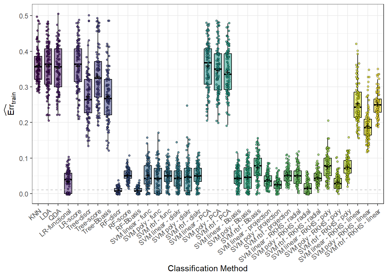

Figure 1.26: Box plots of training errors for 100 simulations for individual classification methods. Mean values are marked with black $+$ symbols.

Code

# dev.off()

Code

# For test data
sub_methods <- methods[c(1:5, 9:32)]

SIMULACE$test |> 
  pivot_longer(cols = methods, names_to = 'method', values_to = 'Err') |>
  mutate(method = factor(method, levels = methods, labels = methods)) |> 
  as.data.frame() |>
    filter(method %in% sub_methods) |>
  ggplot(aes(x = method, y = Err, fill = method, colour = method, alpha = method)) + 
    geom_jitter(position = position_jitter(height = 0, width = 0.15), alpha = 0.6, size = 0.9, pch = 21,
              colour = "black") +
  geom_boxplot(outlier.colour = "white", outlier.shape = 16, outlier.size = 0, 
               notch = FALSE, colour = 'black') + 
  theme_bw() + 
  labs(x = 'Classification Method',
       y = expression(widehat(Err)[test])
       # y = '$\\widehat{\\textnormal{Err}}_{test}$'
       ) + 
  theme(legend.position = 'none',
        axis.text.x = element_text(angle = 45, hjust = 1)) +
  stat_summary(fun = "mean", geom = "point", shape = 4,
               size = 2, color = "black", alpha = 1) +
  scale_x_discrete(labels = methods_names1) +
  theme(plot.margin = unit(c(0.1, 0.1, 0.7, 0.5), "cm")) +
  scale_fill_manual(values = box_col1) +
  scale_alpha_manual(values = box_alpha1) +
  geom_hline(yintercept = min(SIMULACE.df$Err.test), 
             linetype = 'dashed', colour = 'gray20', alpha = 0.8)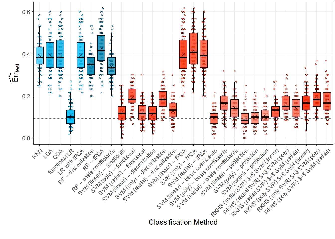

Figure 1.27: Box plots of test errors for 100 simulations for individual classification methods. Mean values are marked with black $+$ symbols.

Code

# ggsave("figures/sim_01_boxplot_test_final.tex", device = tikz, width = 7, height = 5)

We would now like to formally test whether some classification methods are better than others based on the previous simulation on these data, or to show that we can consider them equally successful.

Code

# Check normality
library(nortest)
lillie.test(SIMULACE$test[, 'LR_functional'])$p.value

## [1] 0.008072969

Code

lillie.test(SIMULACE$test[, 'SVM linear - projection'])$p.value

## [1] 0.0004162642

Given the violation of the normality assumption, we cannot use the classic paired t-test. Instead, we will utilize its nonparametric alternative - the paired Wilcoxon test. However, we must be careful with interpretation in this case.

Code

wilcox.test(SIMULACE$test[, 'SVM linear - Bbasis'], SIMULACE$test[, 'SVM linear - projection'], alternative = 'two.sided', paired = TRUE)$p.value

## [1] 0.4297988

Code

wilcox.test(SIMULACE$test[, 'LR_functional'], SIMULACE$test[, 'SVM linear - diskr'], alternative = 'two.sided', paired = TRUE)$p.value

## [1] 0.1274886

Code

wilcox.test(SIMULACE$test[, 'SVM linear - projection'], SIMULACE$test[, 'SVM linear - diskr'], alternative = 'two.sided', paired = TRUE)$p.value

## [1] 0.0001353731

Code

wilcox.test(SIMULACE$test[, 'LR_functional'], SIMULACE$test[, 'SVM linear - projection'], alternative = 'two.sided', paired = TRUE)$p.value

## [1] 0.002208014

Comparing SVM with discretization with functional SVM.

Code

wilcox.test(SIMULACE$test[, 'SVM linear - func'], SIMULACE$test[, 'SVM linear - diskr'], alternative = 'two.sided', paired = TRUE)$p.value

## [1] 0.0003004829

Code

wilcox.test(SIMULACE$test[, 'SVM poly - func'], SIMULACE$test[, 'SVM poly - diskr'], alternative = 'two.sided', paired = TRUE)$p.value

## [1] 0.1656051

Code

wilcox.test(SIMULACE$test[, 'SVM rbf - func'], SIMULACE$test[, 'SVM rbf - diskr'], alternative = 'two.sided', paired = TRUE)$p.value

## [1] 0.4878897

Now let’s look at the comparison between functional logistic regression and projection onto the B-spline basis.

Code

wilcox.test(SIMULACE$test[, 'LR_functional'], SIMULACE$test[, 'SVM linear - projection'], alternative = 'greater', paired = TRUE)$p.value

## [1] 0.001104007

Code

wilcox.test(SIMULACE$test[, 'LR_functional'], SIMULACE$test[, 'SVM poly - projection'], alternative = 'greater', paired = TRUE)$p.value

## [1] 0.0471872

Code

wilcox.test(SIMULACE$test[, 'LR_functional'], SIMULACE$test[, 'SVM rbf - projection'], alternative = 'greater', paired = TRUE)$p.value

## [1] 0.1611741

We see that the linear kernel has a statistically significantly lower error rate compared to functional logistic regression ($p$-value 0.001104). On the other hand, for the remaining SVM kernels, we could not demonstrate that the median of their test errors is smaller than the median of fLR.

We might be interested in further comparisons.

Code

# wilcox.test(SIMULACE$test[, 'SVM rbf - RKHS - radial'], SIMULACE$test[, 'SVM linear - diskr'], alternative = 'less', paired = TRUE)$p.value

# wilcox.test(SIMULACE$test[, 'SVM linear - RKHS - radial'], SIMULACE$test[, 'SVM linear - diskr'], alternative = 'less', paired = TRUE)$p.value

wilcox.test(SIMULACE$test[, 'LR_functional'], SIMULACE$test[, 'SVM linear - RKHS - radial'], alternative = 'less', paired = TRUE)$p.value

## [1] 1.797302e-05

Code

# wilcox.test(SIMULACE$test[, 'LR_functional'], SIMULACE$test[, 'SVM rbf - RKHS - poly'], alternative = 'less', paired = TRUE)$p.value

wilcox.test(SIMULACE$test[, 'LR_functional'], SIMULACE$test[, 'SVM rbf - RKHS - radial'], alternative = 'less', paired = TRUE)$p.value

## [1] 9.443463e-08

Code

# wilcox.test(SIMULACE$test[, 'SVM poly - diskr'], SIMULACE$test[, 'SVM poly - Bbasis'], alternative = 'greater', paired = TRUE)$p.value

Now let’s compare the kernels for projection.

Code

wilcox.test(SIMULACE$test[, 'SVM linear - projection'], SIMULACE$test[, 'SVM poly - projection'], alternative = 'less', paired = TRUE)$p.value

## [1] 0.03742462

Code

wilcox.test(SIMULACE$test[, 'SVM rbf - projection'], SIMULACE$test[, 'SVM poly - projection'], alternative = 'greater', paired = TRUE)$p.value

## [1] 0.2798017

Code

wilcox.test(SIMULACE$test[, 'SVM linear - projection'], SIMULACE$test[, 'SVM rbf - projection'], alternative = 'less', paired = TRUE)$p.value

## [1] 0.02379553

Finally, let’s look at which hyperparameter values were the most frequently chosen.

Table 1.10: Medians of hyperparameter values for selected methods, for which some hyperparameter was determined using cross-validation.
	Median hyperparameter value
KNN_K	4.0
nharm	1.0
LR_func_n_basis	13.0
SVM_d_Linear	15.5
SVM_d_Poly	13.0
SVM_d_Radial	11.0
SVM_RKHS_radial_gamma1	5.2
SVM_RKHS_radial_gamma2	3.2
SVM_RKHS_radial_gamma3	1.6
SVM_RKHS_radial_d1	19.0
SVM_RKHS_radial_d2	18.0
SVM_RKHS_radial_d3	15.0
SVM_RKHS_poly_p1	4.0
SVM_RKHS_poly_p2	4.0
SVM_RKHS_poly_p3	4.0
SVM_RKHS_poly_d1	23.0
SVM_RKHS_poly_d2	31.0
SVM_RKHS_poly_d3	31.0
SVM_RKHS_linear_d1	21.0
SVM_RKHS_linear_d2	25.0
SVM_RKHS_linear_d3	25.0

Code

CV_res <- CV_RESULTS |> 
  pivot_longer(cols = CV_RESULTS |> colnames(), names_to = 'method', values_to = 'hyperparameter') |>
  mutate(method = factor(method, 
                         levels = CV_RESULTS |> colnames(), 
                         labels = CV_RESULTS |> colnames(), ordered = TRUE)) |> 
  as.data.frame() 

CV_res |> 
  filter(method %in% c('KNN_K', 'nharm', 'LR_func_n_basis')) |>
  ggplot(aes(x = hyperparameter, #y = after_stat(density),
             fill = method, colour = method)) + 
  geom_histogram(binwidth = 1, alpha = 0.6) + 
  theme_bw() + 
  facet_grid(~method, scales = 'free') +
  labs(x = 'Hyperparameter Values',
       y = 'Absolute Count') + 
  theme(legend.position = 'none')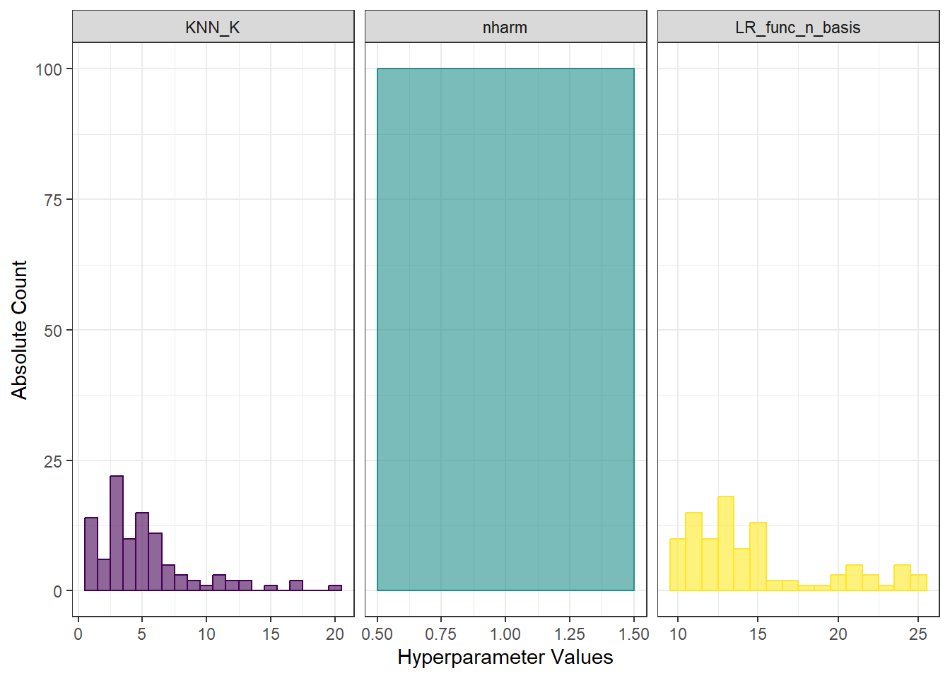

Histograms of hyperparameter values for KNN, functional logistic regression, and a histogram for the number of principal components.

Figure 1.28: Histograms of hyperparameter values for KNN, functional logistic regression, and a histogram for the number of principal components.

Code

CV_res |> 
  filter(method %in% c('SVM_d_Linear', 'SVM_d_Poly', 'SVM_d_Radial')) |>
  ggplot(aes(x = hyperparameter, #y = after_stat(density),
             fill = method, colour = method)) + 
  geom_histogram(binwidth = 5, alpha = 0.6) + 
  theme_bw() + 
  facet_grid(~method, scales = 'free') +
  labs(x = 'Hyperparameter Values',
       y = 'Absolute Count') + 
  theme(legend.position = 'none')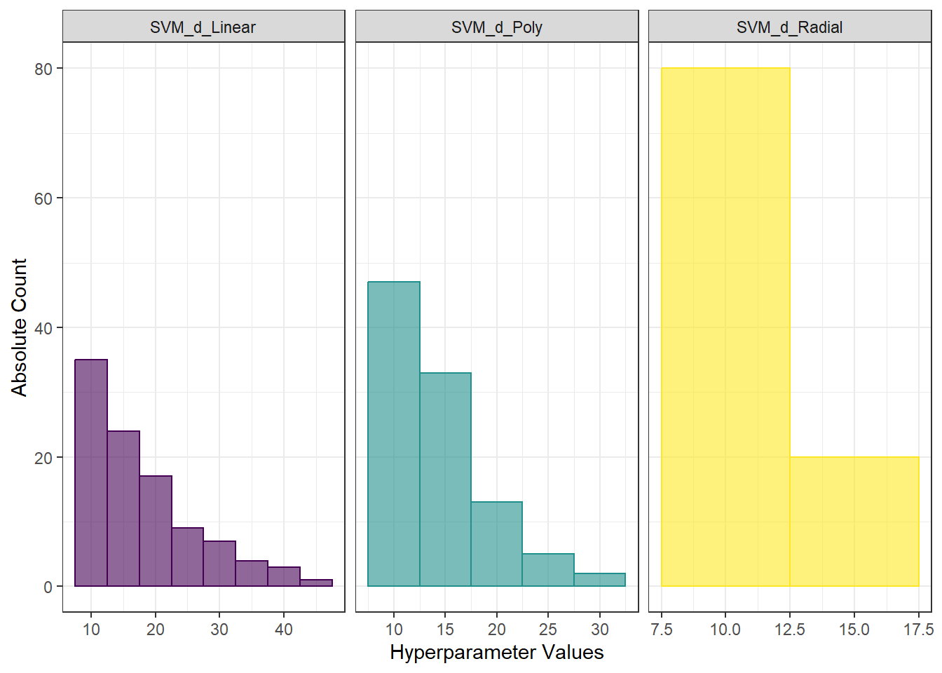

Figure 1.29: Histograms of hyperparameter values for the SVM method with projection onto the B-spline basis.

Code

CV_res |> 
  filter(method %in% c('SVM_RKHS_radial_gamma1', 'SVM_RKHS_radial_gamma2',
                       'SVM_RKHS_radial_gamma3', 'SVM_RKHS_radial_d1', 
                       'SVM_RKHS_radial_d2', 'SVM_RKHS_radial_d3')) |>
  ggplot(aes(x = hyperparameter, #y = after_stat(density),
             fill = method, colour = method)) + 
  geom_histogram(bins = 10, alpha = 0.6) + 
  theme_bw() + 
  facet_wrap(~method, scales = 'free', ncol = 3) +
  labs(x = 'Hyperparameter Values',
       y = 'Absolute Count') + 
  theme(legend.position = 'none')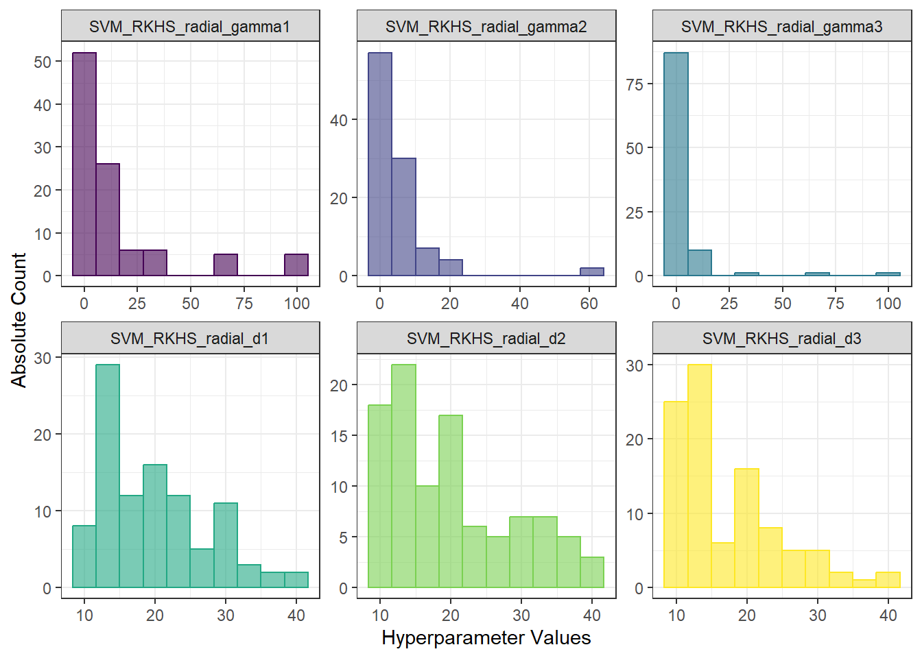

Figure 1.30: Histograms of hyperparameter values for RKHS + SVM with radial kernel.

Code

CV_res |> 
  filter(method %in% c('SVM_RKHS_poly_p1', 'SVM_RKHS_poly_p2',
                       'SVM_RKHS_poly_p3', 'SVM_RKHS_poly_d1',
                       'SVM_RKHS_poly_d2', 'SVM_RKHS_poly_d3')) |>
  ggplot(aes(x = hyperparameter, #y = after_stat(density),
             fill = method, colour = method)) + 
  geom_histogram(binwidth = 1, alpha = 0.6) + 
  theme_bw() + 
  facet_wrap(~method, scales = 'free', ncol = 3) +
  labs(x = 'Hyperparameter Values',
       y = 'Absolute Count') + 
  theme(legend.position = 'none')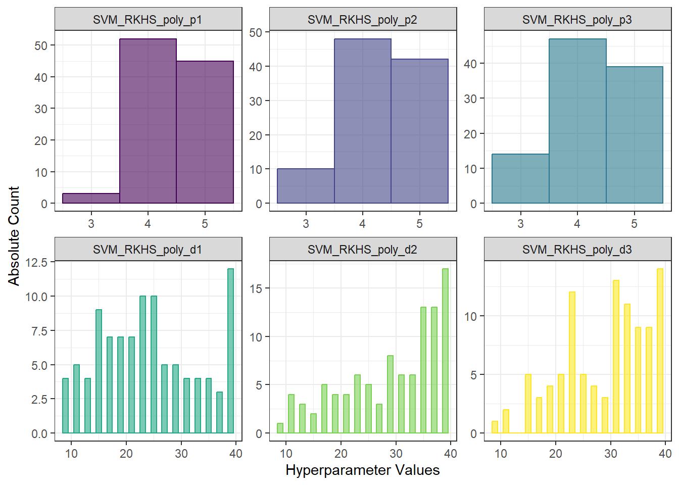

Figure 1.31: Histograms of hyperparameter values for RKHS + SVM with polynomial kernel.

Code

CV_res |> 
  filter(method %in% c('SVM_RKHS_linear_d1',
                       'SVM_RKHS_linear_d2', 'SVM_RKHS_linear_d3')) |>
  ggplot(aes(x = hyperparameter, #y = after_stat(density),
             fill = method, colour = method)) + 
  geom_histogram(binwidth = 5, alpha = 0.6) + 
  theme_bw() + 
  facet_wrap(~method, scales = 'free', ncol = 3) +
  labs(x = 'Hyperparameter Values',
       y = 'Absolute Count') + 
  theme(legend.position = 'none')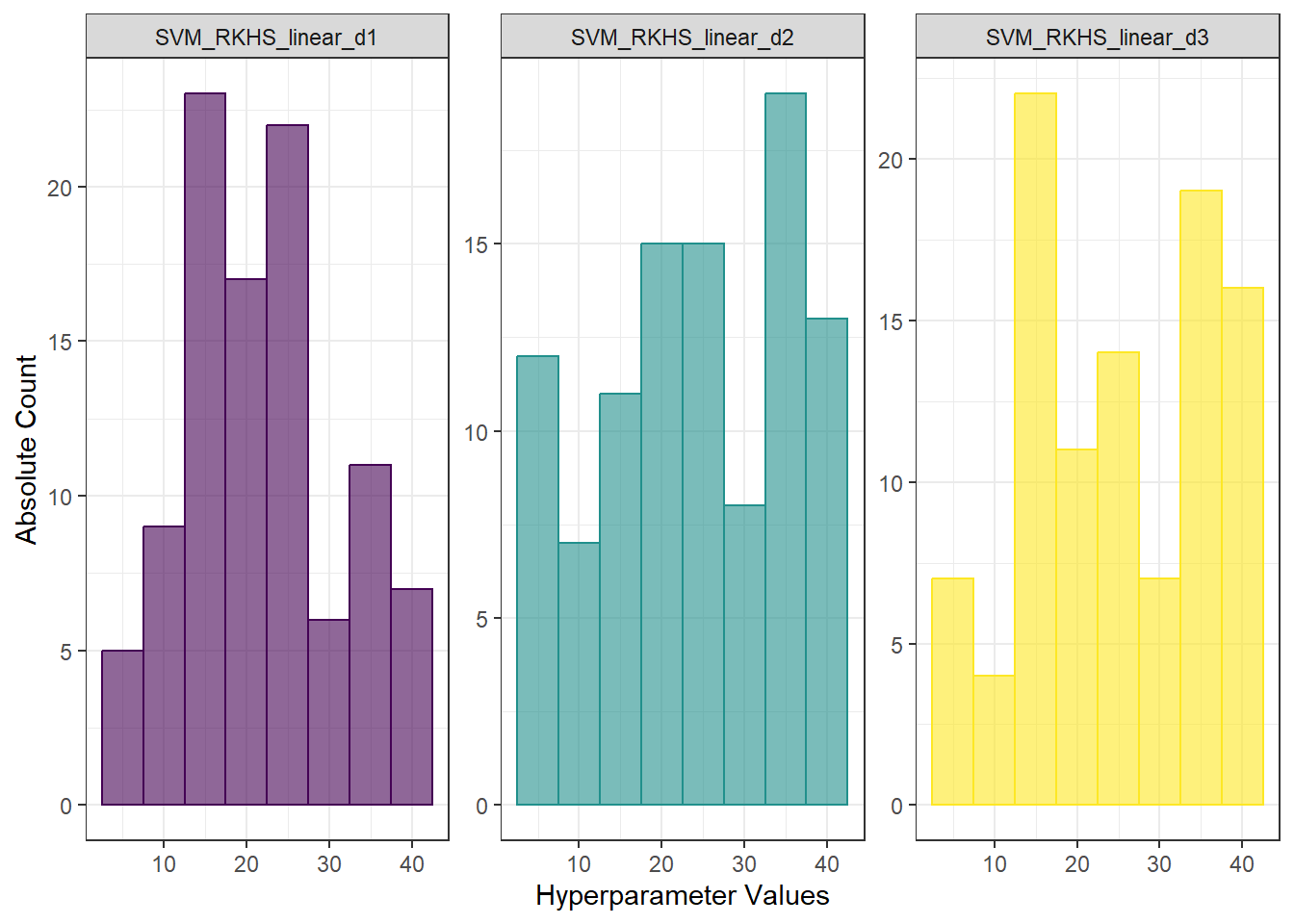

Figure 1.32: Histograms of hyperparameter values for RKHS + SVM with linear kernel.

Muñoz, A. and González, J. (2010) Representing functional data using support vector machines, Pattern Recognition Letters, 31(6), pp. 511–516. doi:10.1016/j.patrec.2009.07.014.↩︎

Support Vector Machine Classification of Functional Data with Random Vertical Shifts

Chapter 1 Classification of simulated curves

1.1 Simulation of Functional Data

1.2 Smoothing Observed Curves

1.3 Classification of Curves

1.3.1 \(K\)-Nearest Neighbors

1.3.2 Linear Discriminant Analysis

1.3.3 Quadratic Discriminant Analysis

1.3.4 Logistic Regression

1.3.4.1 Functional Logistic Regression

1.3.4.2 Logistic Regression with Principal Component Analysis

1.3.5 Decision Trees

1.3.5.1 Interval Discretization

1.3.5.2 Principal Component Scores

1.3.5.3 Basis Coefficients

1.3.6 Random Forests

1.3.6.1 Interval Discretization

1.3.6.2 Principal Component Scores

1.3.6.3 Basis Coefficients

1.3.7 Support Vector Machines

1.3.7.1 SVM for Functional Data

1.3.7.2 Discretization of the Interval

1.3.7.3 Principal Component Scores

1.3.7.4 Basis Coefficients

1.3.7.5 Projection onto the B-spline Basis

1.3.7.6 RKHS + SVM

1.3.7.6.1 Reproducing Kernel Hilbert Space (RKHS)

1.3.7.6.2 Classification Using RKHS

1.3.7.6.3 Implementation of the Method in `R`

1.3.7.6.3.1 Gaussian Kernel

1.3.7.6.3.2 Polynomial Kernel

1.3.7.6.3.3 Linear Kernel

1.3.8 Table of results

1.4 Simulation Study

1.4.1 Results

Chapter 1 Classification of simulated curves

1.1 Simulation of Functional Data

1.2 Smoothing Observed Curves

1.3 Classification of Curves

1.3.1 \(K\)-Nearest Neighbors

1.3.2 Linear Discriminant Analysis

1.3.3 Quadratic Discriminant Analysis

1.3.4 Logistic Regression

1.3.4.1 Functional Logistic Regression

1.3.4.2 Logistic Regression with Principal Component Analysis

1.3.5 Decision Trees

1.3.5.1 Interval Discretization

1.3.5.2 Principal Component Scores

1.3.5.3 Basis Coefficients

1.3.6 Random Forests

1.3.6.1 Interval Discretization

1.3.6.2 Principal Component Scores

1.3.6.3 Basis Coefficients

1.3.7 Support Vector Machines

1.3.7.1 SVM for Functional Data

1.3.7.2 Discretization of the Interval

1.3.7.3 Principal Component Scores

1.3.7.4 Basis Coefficients

1.3.7.5 Projection onto the B-spline Basis

1.3.7.6 RKHS + SVM

1.3.7.6.1 Reproducing Kernel Hilbert Space (RKHS)

1.3.7.6.2 Classification Using RKHS

1.3.7.6.3 Implementation of the Method in R

1.3.7.6.3.1 Gaussian Kernel

1.3.7.6.3.2 Polynomial Kernel

1.3.7.6.3.3 Linear Kernel

1.3.8 Table of results

1.4 Simulation Study

1.4.1 Results

1.3.7.6.3 Implementation of the Method in `R`