Chapter 5 Simulation - Using Derivatives
In this last section concerning simulated data, we will focus on the same data as in Chapter 1 (and possibly also in Chapters 2 or 3), specifically generating functional data from functions calculated using interpolation polynomials. As we generated data with a random vertical shift with a standard deviation parameter \(\sigma_{shift}\) in Section 1, we could attempt to remove this shift and classify the data after its removal. We observed in Section 3 that the accuracy of especially classical classification methods deteriorates rather dramatically as the value of the standard deviation parameter \(\sigma_{shift}\) increases. In contrast, classification methods that account for the functional nature of the data generally behave quite stably, even as \(\sigma_{shift}\) increases.
One way to remove vertical shifts, which we will use in the following section, is to classify data based on the estimate of the first derivative of the generated and smoothed curve, since it is known that \[ \frac{\text d}{\text d t} \big( x(t) + c \big) = \frac{\text d}{\text d t} x(t)= x'(t). \]
5.1 Classification Based on the First Derivative
First, we will simulate functions that we will subsequently want to classify. For simplicity, we will consider two classification classes.
To simulate, we will:
- Choose appropriate functions,
- Generate points from the chosen interval that contain, for example, Gaussian noise,
- Smooth the obtained discrete points into a functional object using a suitable basis system.
This procedure will yield functional objects along with the value of the categorical variable \(Y\), which distinguishes membership in a classification class.
Code
Let’s consider two classification classes, \(Y \in \{0, 1\}\), with the same number of n generated functions for each class. First, we define two functions, each corresponding to one class, on the interval \(I = [0, 6]\).
Now, we will create the functions using interpolation polynomials. First, we define the points through which our curve will pass and then fit an interpolation polynomial through these points, which we will use to generate the curves for classification.
Code
# Defining points for class 0
x.0 <- c(0.00, 0.65, 0.94, 1.42, 2.26, 2.84, 3.73, 4.50, 5.43, 6.00)
y.0 <- c(0, 0.25, 0.86, 1.49, 1.1, 0.15, -0.11, -0.36, 0.23, 0)

# Defining points for class 1
x.1 <- c(0.00, 0.51, 0.91, 1.25, 1.51, 2.14, 2.43, 2.96, 3.70, 4.60,
         5.25, 5.67, 6.00)
y.1 <- c(0.1, 0.4, 0.71, 1.08, 1.47, 1.39, 0.81, 0.05, -0.1, -0.4,
         0.3, 0.37, 0)
Code
Figure 1.1: Points defining both interpolation polynomials.
To calculate the interpolation polynomials, we will use the poly.calc() function from the polynom library. We will also define the functions poly.0() and poly.1(), which will compute the values of the polynomials at a given point in the interval. We will use the predict() function for this, where we input the corresponding polynomial and the point at which we want to evaluate the polynomial.
Code
Code
# Plotting the polynomials
xx <- seq(min(x.0), max(x.0), length = 501)
yy.0 <- poly.0(xx)
yy.1 <- poly.1(xx)

dat_poly_plot <- data.frame(x = c(xx, xx),
                            y = c(yy.0, yy.1),
                            Class = rep(c('Y = 0', 'Y = 1'),
                                        c(length(xx), length(xx))))

ggplot(dat_points, aes(x = x, y = y, colour = Class)) +
  geom_point(size=1.5) +
  theme_bw() +
  geom_line(data = dat_poly_plot,
            aes(x = x, y = y, colour = Class),
            linewidth = 0.8) +
labs(colour = 'Class')![Illustration of two functions on the interval $I = [0, 6]$, from which we generate observations for classes 0 and 1.](05-Simulace_deriv2_files/figure-html/unnamed-chunk-6-1.png)
Figure 1.2: Illustration of two functions on the interval \(I = [0, 6]\), from which we generate observations for classes 0 and 1.
Now, we will create a function to generate random functions with added noise (i.e., points on a predetermined grid) from the chosen generating function. The argument t represents the vector of values at which we want to evaluate the functions, fun denotes the generating function, n is the number of functions, and sigma is the standard deviation \(\sigma\) of the normal distribution \(\text{N}(\mu, \sigma^2)\) from which we randomly generate Gaussian white noise with \(\mu = 0\). To demonstrate the advantage of using methods that work with functional data, we will also add a random component to each simulated observation that represents a vertical shift of the entire function (the parameter sigma_shift). This shift will be generated from a normal distribution with parameter \(\sigma^2 = 4\).
Code
generate_values <- function(t, fun, n, sigma, sigma_shift = 0) {
  # Arguments:
  # t ... vector of values, where the function will be evaluated
  # fun ... generating function of t
  # n ... the number of generated functions / objects
  # sigma ... standard deviation of normal distribution to add noise to data
  # sigma_shift ... parameter of normal distribution for generating shift

  # Value:
  # X ... matrix of dimension length(t) times n with generated values of one
  # function in a column

  X <- matrix(rep(t, times = n), ncol = n, nrow = length(t), byrow = FALSE)
  noise <- matrix(rnorm(n * length(t), mean = 0, sd = sigma),
                  ncol = n, nrow = length(t), byrow = FALSE)
  shift <- matrix(rep(rnorm(n, 0, sigma_shift), each = length(t)),
                  ncol = n, nrow = length(t))
  return(fun(X) + noise + shift)
}
Now we can generate functions. In each of the two classes, we will consider 100 observations, thus n = 100.
Code
We will plot the generated (not yet smoothed) functions colored by class (only the first 10 observations from each class for clarity).
Code
n_curves_plot <- 10 # number of curves we want to plot from each group

DF0 <- cbind(t, X0[, 1:n_curves_plot]) |>
  as.data.frame() |>
  reshape(varying = 2:(n_curves_plot + 1), direction = 'long', sep = '') |>
  subset(select = -id) |>
  mutate(
  time = time - 1,
  group = 0
  )

DF1 <- cbind(t, X1[, 1:n_curves_plot]) |>
  as.data.frame() |>
  reshape(varying = 2:(n_curves_plot + 1), direction = 'long', sep = '') |>
  subset(select = -id) |>
  mutate(
  time = time - 1,
  group = 1
  )

DF <- rbind(DF0, DF1) |>
  mutate(group = factor(group))

DF |> ggplot(aes(x = t, y = V, group = interaction(time, group),
                 colour = group)) +
  geom_line(linewidth = 0.5) +
  theme_bw() +
  labs(x = expression(x[1]),
       y = expression(x[2]),
       colour = 'Class') +
  scale_colour_discrete(labels=c('Y = 0', 'Y = 1'))
Figure 2.1: The first 10 generated observations from each of the two classification classes. The observed data are not smoothed.
5.1.1 Smoothing Observed Curves
Now we will convert the observed discrete values (vectors of values) into functional objects that we will subsequently work with. Again, we will use B-spline basis for smoothing.
We take the entire vector t as knots, and since we consider the first derivative, we choose norder = 5. We will penalize the third derivative of the function, as we now require smooth first derivatives as well.
Code
We will find a suitable value of the smoothing parameter \(\lambda > 0\) using \(GCV(\lambda)\), that is, generalized cross-validation. We will consider the value of \(\lambda\) to be the same for both classification groups, as we would not know in advance which value of $to choose for test observations if different values were chosen for each class.
Code
# combining observations into one matrix
XX <- cbind(X0, X1)

lambda.vect <- 10^seq(from = -3, to = 1, length.out = 50) # vector of lambdas
gcv <- rep(NA, length = length(lambda.vect)) # empty vector for storing GCV

for(index in 1:length(lambda.vect)) {
  curv.Fdpar <- fdPar(bbasis, curv.Lfd, lambda.vect[index])
  BSmooth <- smooth.basis(t, XX, curv.Fdpar) # smoothing
  gcv[index] <- mean(BSmooth$gcv) # average across all observed curves
}

GCV <- data.frame(
  lambda = round(log10(lambda.vect), 3),
  GCV = gcv
)

# find the minimum value
lambda.opt <- lambda.vect[which.min(gcv)]
For better illustration, we will plot the progression of \(GCV(\lambda)\).
Code
GCV |> ggplot(aes(x = lambda, y = GCV)) +
  geom_line(linetype = 'solid', linewidth = 0.6) +
  geom_point(size = 1.5) +
  theme_bw() +
  labs(x = bquote(paste(log[10](lambda), ' ;   ',
                        lambda[optimal] == .(round(lambda.opt, 4)))),
       y = expression(GCV(lambda))) +
  geom_point(aes(x = log10(lambda.opt), y = min(gcv)), colour = 'red', size = 2.5)
## Warning in geom_point(aes(x = log10(lambda.opt), y = min(gcv)), colour = "red", : All aesthetics have length 1, but the data has 50 rows.
## ℹ Please consider using `annotate()` or provide this layer with data containing
## a single row.
Figure 1.5: The progression of \(GCV(\lambda)\) for the chosen vector \(\boldsymbol\lambda\). The x-axis values are plotted on a logarithmic scale. The optimal value of the smoothing parameter \(\lambda_{optimal}\) is shown in red.
With this optimal choice of the smoothing parameter \(\lambda\), we will now smooth all functions and again graphically represent the first 10 observed curves from each classification class.
Code
curv.fdPar <- fdPar(bbasis, curv.Lfd, lambda.opt)
BSmooth <- smooth.basis(t, XX, curv.fdPar)
XXfd <- BSmooth$fd

fdobjSmootheval <- eval.fd(fdobj = XXfd, evalarg = t)
DF$Vsmooth <- c(fdobjSmootheval[, c(1 : n_curves_plot,
                                    (n + 1) : (n + n_curves_plot))])

DF |> ggplot(aes(x = t, y = Vsmooth, group = interaction(time, group),
                 colour = group)) +
  geom_line(linewidth = 0.75) +
  theme_bw() +
  labs(x = expression(x[1]),
       y = expression(x[2]),
       colour = 'Class') +
  scale_colour_discrete(labels=c('Y = 0', 'Y = 1'))
Figure 1.6: The first 10 smoothed curves from each classification class.
Let’s visualize all the smoothed curves along with the mean for each class.
Code
DFsmooth <- data.frame(
  t = rep(t, 2 * n),
  time = rep(rep(1:n, each = length(t)), 2),
  Smooth = c(fdobjSmootheval),
  Mean = c(rep(apply(fdobjSmootheval[ , 1 : n], 1, mean), n),
            rep(apply(fdobjSmootheval[ , (n + 1) : (2 * n)], 1, mean), n)),
  group = factor(rep(c(0, 1), each = n * length(t)))
)

DFmean <- data.frame(
  t = rep(t, 2),
  Mean = c(apply(fdobjSmootheval[ , 1 : n], 1, mean),
            apply(fdobjSmootheval[ , (n + 1) : (2 * n)], 1, mean)),
  group = factor(rep(c(0, 1), each = length(t)))
)

DFsmooth |> ggplot(aes(x = t, y = Smooth, group = interaction(time, group),
                 colour = group)) +
  geom_line(linewidth = 0.25, alpha = 0.5) +
  theme_bw() +
  labs(x = expression(x[1]),
       y = expression(x[2]),
       colour = 'Class') +
  scale_colour_discrete(labels = c('Y = 0', 'Y = 1')) +
  geom_line(aes(x = t, y = Mean, colour = group),
            linewidth = 1.2, linetype = 'solid') +
  scale_x_continuous(expand = c(0.01, 0.01)) +
  #ylim(c(-1, 2)) +
  scale_y_continuous(expand = c(0.01, 0.01)) #, limits = c(-1, 2))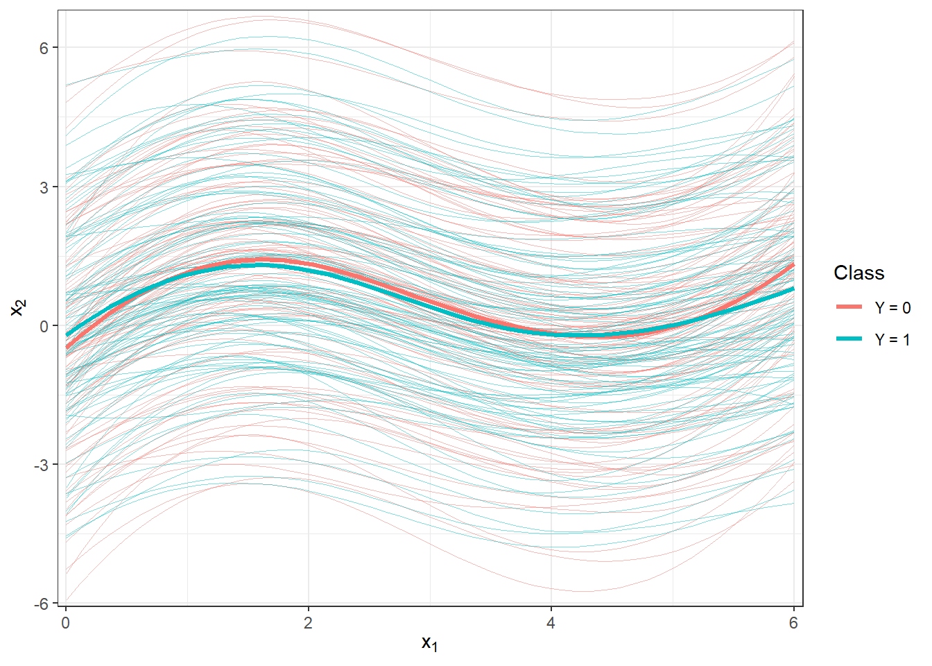
Figure 1.7: Plot of all smoothed observed curves, colored by their classification class. The mean for each class is shown with a thick line.
Code
DFsmooth <- data.frame(
  t = rep(t, 2 * n),
  time = rep(rep(1:n, each = length(t)), 2),
  Smooth = c(fdobjSmootheval),
  Mean = c(rep(apply(fdobjSmootheval[ , 1 : n], 1, mean), n),
            rep(apply(fdobjSmootheval[ , (n + 1) : (2 * n)], 1, mean), n)),
  group = factor(rep(c(0, 1), each = n * length(t)))
)

DFmean <- data.frame(
  t = rep(t, 2),
  Mean = c(apply(fdobjSmootheval[ , 1 : n], 1, mean),
            apply(fdobjSmootheval[ , (n + 1) : (2 * n)], 1, mean)),
  group = factor(rep(c(0, 1), each = length(t)))
)

DFsmooth |> ggplot(aes(x = t, y = Smooth, group = interaction(time, group),
                 colour = group)) +
  geom_line(linewidth = 0.25, alpha = 0.5) +
  theme_bw() +
  labs(x = expression(x[1]),
       y = expression(x[2]),
       colour = 'Class') +
  scale_colour_discrete(labels = c('Y = 0', 'Y = 1')) +
  geom_line(aes(x = t, y = Mean, colour = group),
            linewidth = 1.2, linetype = 'solid') +
  scale_x_continuous(expand = c(0.01, 0.01)) +
  #ylim(c(-1, 2)) +
  scale_y_continuous(expand = c(0.01, 0.01), limits = c(-1, 2))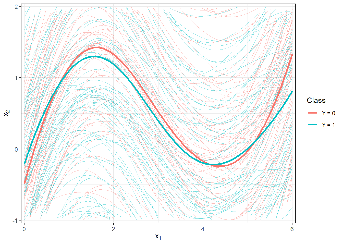
Figure 2.2: Plot of all smoothed observed curves, colored by their classification class. The mean for each class is shown with a thick line. Zoomed view.
5.1.2 Calculation of Derivatives
To compute the derivative for the functional object, we will use the deriv.fd() function from the fda package in R. Since we want to classify based on the first derivative, we choose the argument Lfdobj = 1.
Now let’s plot the first few first derivatives for both classification classes. Notice from the figure below that the vertical shift due to differentiation has indeed been successfully removed. However, we have somewhat lost the distinctiveness between the curves because, as implied by the figure, the derivative curves for both classes differ primarily towards the end of the interval, specifically for the argument in the range approximately \([5, 6]\).
Code
fdobjSmootheval <- eval.fd(fdobj = XXder, evalarg = t)
DF$Vsmooth <- c(fdobjSmootheval[, c(1 : n_curves_plot,
                                    (n + 1) : (n + n_curves_plot))])

DF |> ggplot(aes(x = t, y = Vsmooth, group = interaction(time, group),
                 colour = group)) +
  geom_line(linewidth = 0.75) +
  theme_bw() +
  labs(x = expression(x[1]),
       y = expression(x[2]),
       colour = 'Class') +
  scale_colour_discrete(labels=c('Y = 0', 'Y = 1'))
Let’s also illustrate all curves including the average separately for each class.
Code
abs.labs <- paste("Classification class:", c("$Y = 0$", "$Y = 1$"))
names(abs.labs) <- c('0', '1')

# fdobjSmootheval <- eval.fd(fdobj = XXfd, evalarg = t)

DFsmooth <- data.frame(
  t = rep(t, 2 * n),
  time = rep(rep(1:n, each = length(t)), 2),
  Smooth = c(fdobjSmootheval),
  group = factor(rep(c(0, 1), each = n * length(t)))
)

DFmean <- data.frame(
  t = rep(t, 2),
  Mean = c(eval.fd(fdobj = mean.fd(XXder[1:n]), evalarg = t),
           eval.fd(fdobj = mean.fd(XXder[(n + 1):(2 * n)]), evalarg = t)),
  group = factor(rep(c(0, 1), each = length(t)))
)

DFsmooth |> ggplot(aes(x = t, y = Smooth, #group = interaction(time, group),
                 colour = group)) +
  geom_line(aes(group = time), linewidth = 0.05, alpha = 0.5) +
  theme_bw() +
  labs(x = "$t$",
       # y = "$\\frac{\\text d}{\\text d t} x_i(t)$",
       y ="$x_i'(t)$",
       colour = 'Class') +
  # geom_line(data = DFsmooth |>
  #             mutate(group = factor(ifelse(group == '0', '1', '0'))) |>
  #             filter(group == '1'),
  #           aes(x = t, y = Mean, colour = group),
  #           colour = 'tomato', linewidth = 0.8, linetype = 'solid') +
  # geom_line(data = DFsmooth |>
  #             mutate(group = factor(ifelse(group == '0', '1', '0'))) |>
  #             filter(group == '0'),
  #           aes(x = t, y = Mean, colour = group),
  #           colour = 'deepskyblue2', linewidth = 0.8, linetype = 'solid') +
  geom_line(data = DFmean |>
              mutate(group = factor(ifelse(group == '0', '1', '0'))),
            aes(x = t, y = Mean, colour = group),
            colour = 'grey2', linewidth = 0.8, linetype = 'dashed') +
  geom_line(data = DFmean, aes(x = t, y = Mean, colour = group),
            colour = 'grey2', linewidth = 1.25, linetype = 'solid') +
  scale_x_continuous(expand = c(0.01, 0.01)) +
  facet_wrap(~group, labeller = labeller(group = abs.labs)) +
  scale_y_continuous(expand = c(0.02, 0.02)) +
  theme(legend.position = 'none',
        plot.margin = unit(c(0.1, 0.1, 0.3, 0.5), "cm")) +
  coord_cartesian(ylim = c(-1.4, 3.5)) +
  scale_colour_manual(values = c('tomato', 'deepskyblue2'))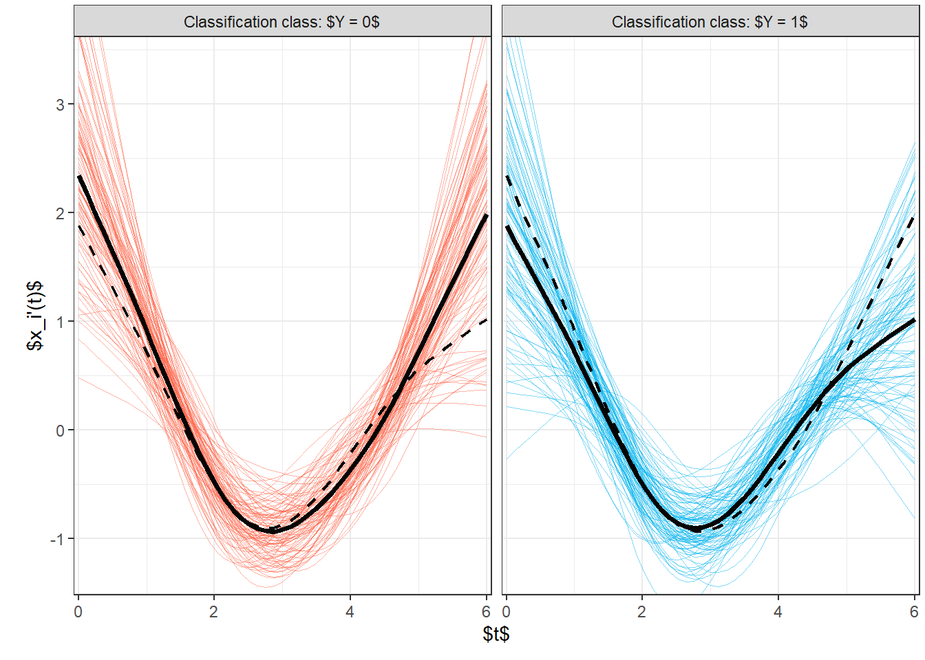
Figure 5.1: Plot of all smoothed observed curves, colored differently according to classification class membership. The average for each class is plotted as a solid black line.
Code
DFsmooth <- data.frame(
  t = rep(t, 2 * n),
  time = rep(rep(1:n, each = length(t)), 2),
  Smooth = c(fdobjSmootheval),
  Mean = c(rep(apply(fdobjSmootheval[ , 1 : n], 1, mean), n),
            rep(apply(fdobjSmootheval[ , (n + 1) : (2 * n)], 1, mean), n)),
  group = factor(rep(c(0, 1), each = n * length(t)))
)

DFmean <- data.frame(
  t = rep(t, 2),
  Mean = c(apply(fdobjSmootheval[ , 1 : n], 1, mean),
            apply(fdobjSmootheval[ , (n + 1) : (2 * n)], 1, mean)),
  group = factor(rep(c(0, 1), each = length(t)))
)

DFsmooth |> ggplot(aes(x = t, y = Smooth, group = interaction(time, group),
                 colour = group)) +
  geom_line(linewidth = 0.25, alpha = 0.5) +
  theme_bw() +
  labs(x = expression(x[1]),
       y = expression(x[2]),
       colour = 'Class') +
  scale_colour_discrete(labels = c('Y = 0', 'Y = 1')) +
  geom_line(aes(x = t, y = Mean), colour = 'grey3',
            linewidth = 0.7, linetype = 'dashed') +
  scale_x_continuous(expand = c(0.01, 0.01)) +
  #ylim(c(-1, 2)) +
  scale_y_continuous(expand = c(0.01, 0.01), limits = c(-1.5, 2))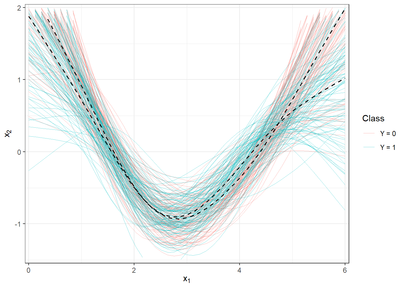
Figure 5.2: Plot of all smoothed observed curves, colored differently according to classification class membership. The average for each class is plotted as a solid black line. Closer look.
5.1.3 Classification of Curves
First, we will load the necessary libraries for classification.
Code
library(caTools) # for splitting into test and training sets
library(caret) # for k-fold CV
library(fda.usc) # for KNN, fLR
library(MASS) # for LDA
library(fdapace)
library(pracma)
library(refund) # for logistic regression on scores
library(nnet) # for logistic regression on scores
library(caret)
library(rpart) # decision trees
library(rattle) # visualization
library(e1071)
library(randomForest) # random forest
To compare individual classifiers, we will split the generated observations into two parts in a 70:30 ratio for training and testing (validation) sets. The training set will be used to construct the classifier, while the test set will be used to calculate the classification error and potentially other characteristics of our model. The resulting classifiers can then be compared based on these computed characteristics in terms of their classification success.
Code
Next, we will examine the representation of individual groups in the test and training portions of the data.
## Y.train
##  0  1
## 71 69## Y.test
## 0 1
## 29 31## Y.train
## 0 1
## 0.5071429 0.4928571## Y.test
## 0 1
## 0.4833333 0.51666675.1.3.1 \(K\) Nearest Neighbors
Let’s start with a non-parametric classification method, specifically the \(K\) nearest neighbors method. First, we will create the necessary objects so that we can work with them using the classif.knn() function from the fda.usc library.
Now we can define the model and look at its classification success. The last question remains how to choose the optimal number of neighbors \(K\). We could choose this number as the value of \(K\) that results in the minimum error rate on the training data. However, this could lead to overfitting the model, so we will use cross-validation. Given the computational complexity and size of the dataset, we will opt for \(k\)-fold CV; we will choose a value of \(k = 10\).
Code
# model for all training data for K = 1, 2, ..., sqrt(n_train)
neighb.model <- classif.knn(group = y.train,
fdataobj = x.train,
knn = c(1:round(sqrt(length(y.train)))))
# summary(neighb.model) # summary of the model
# plot(neighb.model$gcv, pch = 16) # plot GCV dependence on the number of neighbors K
# neighb.model$max.prob # maximum accuracy
(K.opt <- neighb.model$h.opt) # optimal value of K## [1] 12Let’s proceed with the previous procedure for the training data, which we will split into \(k\) parts and repeat this code \(k\) times.
Code
k_cv <- 10 # k-fold CV
neighbours <- c(1:(2 * ceiling(sqrt(length(y.train))))) # number of neighbors
# split training data into k parts
folds <- createMultiFolds(X.train$fdnames$reps, k = k_cv, time = 1)
# empty matrix to store the results
# columns will contain accuracy values for the corresponding part of the training set
# rows will contain values for the given number of neighbors K
CV.results <- matrix(NA, nrow = length(neighbours), ncol = k_cv)
for (index in 1:k_cv) {
# define the current index set
fold <- folds[[index]]
x.train.cv <- subset(X.train, c(1:length(X.train$fdnames$reps)) %in% fold) |>
fdata()
y.train.cv <- subset(Y.train, c(1:length(X.train$fdnames$reps)) %in% fold) |>
factor() |> as.numeric()
x.test.cv <- subset(X.train, !c(1:length(X.train$fdnames$reps)) %in% fold) |>
fdata()
y.test.cv <- subset(Y.train, !c(1:length(X.train$fdnames$reps)) %in% fold) |>
factor() |> as.numeric()
# iterate over each part ... repeat k times
for(neighbour in neighbours) {
# model for specific choice of K
neighb.model <- classif.knn(group = y.train.cv,
fdataobj = x.train.cv,
knn = neighbour)
# predictions on validation set
model.neighb.predict <- predict(neighb.model,
new.fdataobj = x.test.cv)
# accuracy on validation set
accuracy <- table(y.test.cv, model.neighb.predict) |>
prop.table() |> diag() |> sum()
# store accuracy in the position for given K and fold
CV.results[neighbour, index] <- accuracy
}
}
# compute average accuracies for individual K across folds
CV.results <- apply(CV.results, 1, mean)
K.opt <- which.max(CV.results)
presnost.opt.cv <- max(CV.results)
# CV.resultsWe can see that the best value for the parameter \(K\) is 14, with an error rate calculated using 10-fold CV of 0.2594.
For clarity, let’s also plot the validation error rate as a function of the number of neighbors \(K\).
Code
CV.results <- data.frame(K = neighbours, CV = CV.results)
CV.results |> ggplot(aes(x = K, y = 1 - CV)) +
geom_line(linetype = 'dashed', colour = 'grey') +
geom_point(size = 1.5) +
geom_point(aes(x = K.opt, y = 1 - presnost.opt.cv), colour = 'red', size = 2) +
theme_bw() +
labs(x = bquote(paste(K, ' ; ',
K[optimal] == .(K.opt))),
y = 'Validation Error Rate') +
scale_x_continuous(breaks = neighbours)## Warning in geom_point(aes(x = K.opt, y = 1 - presnost.opt.cv), colour = "red", : All aesthetics have length 1, but the data has 24 rows.
## ℹ Please consider using `annotate()` or provide this layer with data containing
## a single row.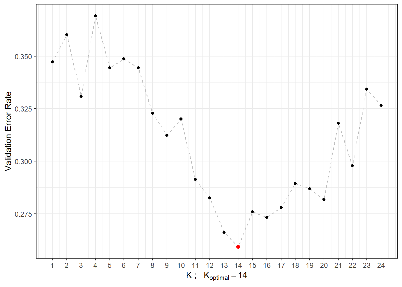
Figure 5.3: Dependency of validation error rate on the value of \(K\), i.e., on the number of neighbors.
Now that we have determined the optimal value of the parameter \(K\), we can build the final model.
Code
neighb.model <- classif.knn(group = y.train, fdataobj = x.train, knn = K.opt)
# predictions
model.neighb.predict <- predict(neighb.model,
new.fdataobj = fdata(X.test))
# summary(neighb.model)
# accuracy on test data
accuracy <- table(as.numeric(factor(Y.test)), model.neighb.predict) |>
prop.table() |>
diag() |>
sum()
# error rate
# 1 - accuracyThus, the error rate of the model constructed using the \(K\)-nearest neighbors method with the optimal choice of \(K_{optimal}\) equal to 14, determined by cross-validation, is 0.3071 on the training data and 0.1833 on the test data.
To compare different models, we can use both types of error rates, which we will store in a table for clarity.
5.1.3.2 Linear Discriminant Analysis
As the second method for constructing a classifier, we will consider Linear Discriminant Analysis (LDA). Since this method cannot be applied to functional data, we must first discretize the data, which we will do using Functional Principal Component Analysis (FPCA). We will then perform the classification algorithm on the scores of the first \(p\) principal components. We will choose the number of components \(p\) such that the first \(p\) principal components together explain at least 90% of the variability in the data.
First, let’s perform the functional principal component analysis and determine the number \(p\).
Code
# principal component analysis
data.PCA <- pca.fd(X.train, nharm = 10) # nharm - maximum number of PCs
nharm <- which(cumsum(data.PCA$varprop) >= 0.9)[1] # determine p
if(nharm == 1) nharm <- 2
data.PCA <- pca.fd(X.train, nharm = nharm)
data.PCA.train <- as.data.frame(data.PCA$scores) # scores of the first p PCs
data.PCA.train$Y <- factor(Y.train) # class membershipIn this particular case, we took the number of principal components as \(p\) = 3, which together explain 93.96 % of the variability in the data. The first principal component explains 50.6 % and the second 33.44 % of the variability. We can graphically display the scores of the first two principal components, color-coded according to class membership.
Code
data.PCA.train |> ggplot(aes(x = V1, y = V2, colour = Y)) +
geom_point(size = 1.5) +
labs(x = paste('1st Principal Component (explained variability',
round(100 * data.PCA$varprop[1], 2), '%)'),
y = paste('2nd Principal Component (',
round(100 * data.PCA$varprop[2], 2), '%)'),
colour = 'Group') +
scale_colour_discrete(labels = c('Y = 0', 'Y = 1')) +
theme_bw()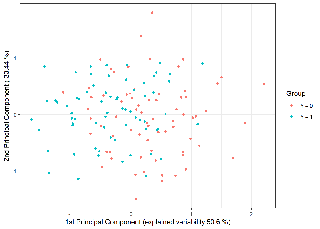
Figure 5.4: Scores of the first two principal components for the training data. Points are color-coded according to class membership.
To determine the classification accuracy on the test data, we need to calculate the scores for the first 3 principal components for the test data. These scores are determined using the formula:
\[ \xi_{i, j} = \int \left( X_i(t) - \mu(t)\right) \cdot \rho_j(t)\text{ dt}, \]
where \(\mu(t)\) is the mean function and \(\rho_j(t)\) is the eigenfunction (functional principal component).
Code
# compute scores for test functions
scores <- matrix(NA, ncol = nharm, nrow = length(Y.test)) # empty matrix
for(k in 1:dim(scores)[1]) {
xfd = X.test[k] - data.PCA$meanfd[1] # k-th observation - mean function
scores[k, ] = inprod(xfd, data.PCA$harmonics)
# scalar product of residuals and eigenfunctions (functional principal components)
}
data.PCA.test <- as.data.frame(scores)
data.PCA.test$Y <- factor(Y.test)
colnames(data.PCA.test) <- colnames(data.PCA.train) Now we can construct the classifier on the training portion of the data.
Code
# model
clf.LDA <- lda(Y ~ ., data = data.PCA.train)
# accuracy on training data
predictions.train <- predict(clf.LDA, newdata = data.PCA.train)
accuracy.train <- table(data.PCA.train$Y, predictions.train$class) |>
prop.table() |> diag() |> sum()
# accuracy on test data
predictions.test <- predict(clf.LDA, newdata = data.PCA.test)
accuracy.test <- table(data.PCA.test$Y, predictions.test$class) |>
prop.table() |> diag() |> sum()We have calculated the error rate of the classifier on the training (31.43 %) and on the test data (23.33 %).
To visually represent the method, we can indicate the decision boundary in the plot of the scores of the first two principal components. We will compute this boundary on a dense grid of points and display it using the geom_contour() function.
Code
# add decision boundary
np <- 1001 # number of grid points
# x-axis ... 1st PC
nd.x <- seq(from = min(data.PCA.train$V1),
to = max(data.PCA.train$V1), length.out = np)
# y-axis ... 2nd PC
nd.y <- seq(from = min(data.PCA.train$V2),
to = max(data.PCA.train$V2), length.out = np)
# case for 2 PCs ... p = 2
nd <- expand.grid(V1 = nd.x, V2 = nd.y)
# if p = 3
if(dim(data.PCA.train)[2] == 4) {
nd <- expand.grid(V1 = nd.x, V2 = nd.y, V3 = data.PCA.train$V3[1])}
# if p = 4
if(dim(data.PCA.train)[2] == 5) {
nd <- expand.grid(V1 = nd.x, V2 = nd.y, V3 = data.PCA.train$V3[1],
V4 = data.PCA.train$V4[1])}
# if p = 5
if(dim(data.PCA.train)[2] == 6) {
nd <- expand.grid(V1 = nd.x, V2 = nd.y, V3 = data.PCA.train$V3[1],
V4 = data.PCA.train$V4[1], V5 = data.PCA.train$V5[1])}
# add Y = 0, 1
nd <- nd |> mutate(prd = as.numeric(predict(clf.LDA, newdata = nd)$class))
data.PCA.train |> ggplot(aes(x = V1, y = V2, colour = Y)) +
geom_point(size = 1.5) +
labs(x = paste('1st Principal Component (explained variability',
round(100 * data.PCA$varprop[1], 2), '%)'),
y = paste('2nd Principal Component (',
round(100 * data.PCA$varprop[2], 2), '%)'),
colour = 'Group') +
scale_colour_discrete(labels = c('Y = 0', 'Y = 1')) +
theme_bw() +
geom_contour(data = nd, aes(x = V1, y = V2, z = prd), colour = 'black')
Figure 1.11: Scores of the first two principal components, color-coded according to class membership. The decision boundary (line in the plane of the first two principal components) between the classes constructed using LDA is marked in black.
We see that the decision boundary is a line, a linear function in the 2D space, which is indeed what we expected from LDA. Finally, we will add the error rates to the summary table.
5.1.3.3 Quadratic Discriminant Analysis
Next, we will construct a classifier using Quadratic Discriminant Analysis (QDA). This is an analogous case to LDA, with the difference that we now allow for different covariance matrices for each of the classes from which the corresponding scores are drawn. This relaxed assumption of equal covariance matrices leads to a quadratic boundary between the classes.
In R, we perform QDA similarly to how we did LDA in the previous section. We will compute the scores for the training and test functions using the results from the functional Principal Component Analysis (PCA) obtained earlier.
Thus, we can proceed directly to constructing the classifier using the qda() function. We will then calculate the accuracy of the classifier on both test and training data.
Code
# model
clf.QDA <- qda(Y ~ ., data = data.PCA.train)
# accuracy on training data
predictions.train <- predict(clf.QDA, newdata = data.PCA.train)
accuracy.train <- table(data.PCA.train$Y, predictions.train$class) |>
prop.table() |> diag() |> sum()
# accuracy on test data
predictions.test <- predict(clf.QDA, newdata = data.PCA.test)
accuracy.test <- table(data.PCA.test$Y, predictions.test$class) |>
prop.table() |> diag() |> sum()We have calculated the error rate of the classifier on the training (35 %) and test data (20 %).
To visually represent the method, we can indicate the decision boundary in the plot of the scores of the first two principal components. We will compute this boundary on a dense grid of points and display it using the geom_contour() function, just like in the case of LDA.
Code
nd <- nd |> mutate(prd = as.numeric(predict(clf.QDA, newdata = nd)$class))
data.PCA.train |> ggplot(aes(x = V1, y = V2, colour = Y)) +
geom_point(size = 1.5) +
labs(x = paste('1st Principal Component (explained variability',
round(100 * data.PCA$varprop[1], 2), '%)'),
y = paste('2nd Principal Component (',
round(100 * data.PCA$varprop[2], 2), '%)'),
colour = 'Group') +
scale_colour_discrete(labels = c('Y = 0', 'Y = 1')) +
theme_bw() +
geom_contour(data = nd, aes(x = V1, y = V2, z = prd), colour = 'black')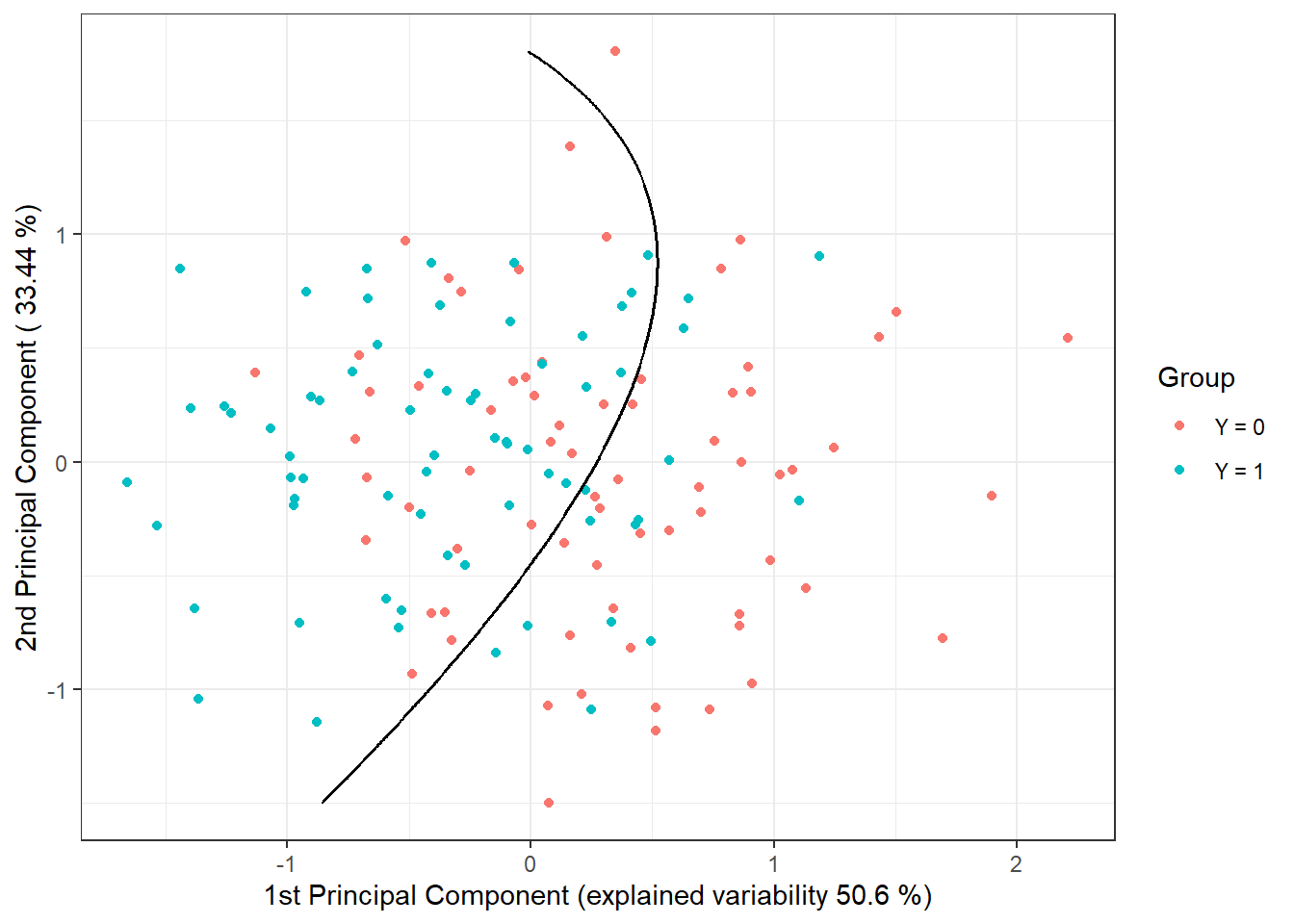
Figure 4.1: Scores of the first two principal components, color-coded according to class membership. The decision boundary (parabola in the plane of the first two principal components) between the classes constructed using QDA is marked in black.
Notice that the decision boundary between the classification classes is now a parabola.
Finally, we will add the error rates to the summary table.
5.1.3.4 Logistic Regression
We can perform logistic regression in two ways. First, we can use the functional analogue of classical logistic regression, and second, we can apply classical multivariate logistic regression on the scores of the first \(p\) principal components.
5.1.3.4.1 Functional Logistic Regression
Analogous to the case with finite-dimensional input data, we consider the logistic model in the form:
\[ g\left(\mathbb E [Y|X = x]\right) = \eta (x) = g(\pi(x)) = \alpha + \int \beta(t)\cdot x(t) \text d t, \]
where \(\eta(x)\) is a linear predictor taking values in the interval \((-\infty, \infty)\), \(g(\cdot)\) is the link function (in the case of logistic regression, this is the logit function \(g: (0,1) \rightarrow \mathbb R,\ g(p) = \ln\frac{p}{1-p}\)), and \(\pi(x)\) is the conditional probability:
\[ \pi(x) = \text{Pr}(Y = 1 | X = x) = g^{-1}(\eta(x)) = \frac{\text e^{\alpha + \int \beta(t)\cdot x(t) \text d t}}{1 + \text e^{\alpha + \int \beta(t)\cdot x(t) \text d t}}, \]
where \(\alpha\) is a constant and \(\beta(t) \in L^2[a, b]\) is a parametric function. Our goal is to estimate this parametric function.
For functional logistic regression, we will use the fregre.glm() function from the fda.usc package. First, we will create suitable objects for the classifier construction.
Code
To estimate the parametric function \(\beta(t)\), we need to express it in some basis representation, in our case, a B-spline basis. However, we need to determine a suitable number of basis functions. We could determine this based on the error rate on the training data, but this would lead to a preference for selecting a large number of bases, resulting in overfitting.
Let us illustrate this with the following case. For each number of bases \(n_{basis} \in \{4, 5, \dots, 50\}\), we will train the model on the training data, determine the error rate on the training data, and also calculate the error rate on the test data. We must remember that we cannot use the same data for estimating the test error rate, as this would underestimate the error rate.
Code
n.basis.max <- 50
n.basis <- 4:n.basis.max
pred.baz <- matrix(NA, nrow = length(n.basis), ncol = 2,
dimnames = list(n.basis, c('Err.train', 'Err.test')))
for (i in n.basis) {
# basis for betas
basis2 <- create.bspline.basis(rangeval = range(tt), nbasis = i)
# formula
f <- Y ~ x
# basis for x and betas
basis.x <- list("x" = basis1) # smoothed data
basis.b <- list("x" = basis2)
# input data for the model
ldata <- list("df" = dataf, "x" = x.train)
# binomial model ... logistic regression model
model.glm <- fregre.glm(f, family = binomial(), data = ldata,
basis.x = basis.x, basis.b = basis.b)
# accuracy on training data
predictions.train <- predict(model.glm, newx = ldata)
predictions.train <- data.frame(Y.pred = ifelse(predictions.train < 1/2, 0, 1))
accuracy.train <- table(Y.train, predictions.train$Y.pred) |>
prop.table() |> diag() |> sum()
# accuracy on test data
newldata = list("df" = as.data.frame(Y.test), "x" = fdata(X.test))
predictions.test <- predict(model.glm, newx = newldata)
predictions.test <- data.frame(Y.pred = ifelse(predictions.test < 1/2, 0, 1))
accuracy.test <- table(Y.test, predictions.test$Y.pred) |>
prop.table() |> diag() |> sum()
# insert into the matrix
pred.baz[as.character(i), ] <- 1 - c(accuracy.train, accuracy.test)
}
pred.baz <- as.data.frame(pred.baz)
pred.baz$n.basis <- n.basisLet’s visualize the trends of both training and test error rates in a graph based on the number of basis functions.
Code
n.basis.beta.opt <- pred.baz$n.basis[which.min(pred.baz$Err.test)]
pred.baz |> ggplot(aes(x = n.basis, y = Err.test)) +
geom_line(linetype = 'dashed', colour = 'black') +
geom_line(aes(x = n.basis, y = Err.train), colour = 'deepskyblue3',
linetype = 'dashed', linewidth = 0.5) +
geom_point(size = 1.5) +
geom_point(aes(x = n.basis, y = Err.train), colour = 'deepskyblue3',
size = 1.5) +
geom_point(aes(x = n.basis.beta.opt, y = min(pred.baz$Err.test)),
colour = 'red', size = 2) +
theme_bw() +
labs(x = bquote(paste(n[basis], ' ; ',
n[optimal] == .(n.basis.beta.opt))),
y = 'Error Rate')## Warning: Use of `pred.baz$Err.test` is discouraged.
## ℹ Use `Err.test` instead.## Warning in geom_point(aes(x = n.basis.beta.opt, y = min(pred.baz$Err.test)), : All aesthetics have length 1, but the data has 47 rows.
## ℹ Please consider using `annotate()` or provide this layer with data containing
## a single row.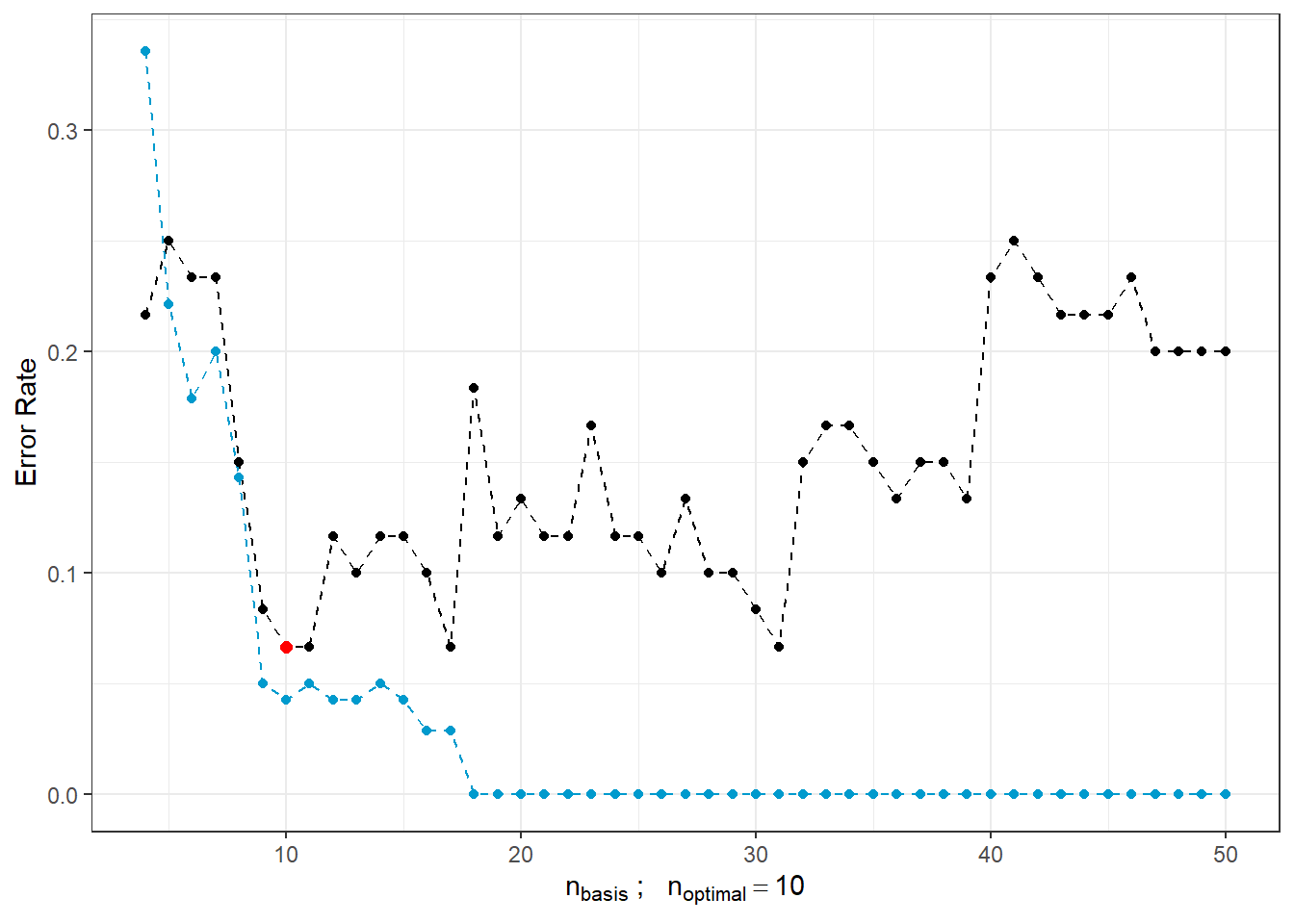
Figure 1.13: Dependence of test and training error rates on the number of basis functions for \(\beta\). The red point represents the optimal number \(n_{optimal}\) chosen as the minimum test error rate, the black line depicts the test error, and the blue dashed line illustrates the training error rate.
We see that as the number of bases for \(\beta(t)\) increases, the training error rate (represented by the blue line) tends to decrease, suggesting that we might choose large values for \(n_{basis}\) based solely on it. In contrast, the optimal choice based on the test error rate is \(n\) equal to 10, which is significantly smaller than 50. Conversely, as \(n\) increases, the test error rate rises, indicating overfitting of the model.
For these reasons, we will use 10-fold cross-validation to determine the optimal number of basis functions for \(\beta(t)\). The maximum number of basis functions considered is 35, as we observed that exceeding this value leads to overfitting.
Code
### 10-fold cross-validation
n.basis.max <- 35
n.basis <- 4:n.basis.max
k_cv <- 10 # k-fold CV
# divide the training data into k parts
folds <- createMultiFolds(X.train$fdnames$reps, k = k_cv, time = 1)
## elements that do not change during the loop
# points at which the functions are evaluated
tt <- x.train[["argvals"]]
rangeval <- range(tt)
# B-spline basis
basis1 <- X.train$basis
# formula
f <- Y ~ x
# basis for x
basis.x <- list("x" = basis1)
# empty matrix to store results
# columns will contain accuracy values for the respective training subset
# rows will contain values for the respective number of bases
CV.results <- matrix(NA, nrow = length(n.basis), ncol = k_cv,
dimnames = list(n.basis, 1:k_cv))Now that we have everything prepared, we will calculate the error rates for each of the ten subsets of the training set. Subsequently, we will determine the average error and take the argument of the minimum validation error as the optimal \(n\).
Code
for (index in 1:k_cv) {
# define the index set
fold <- folds[[index]]
x.train.cv <- subset(X.train, c(1:length(X.train$fdnames$reps)) %in% fold) |>
fdata()
y.train.cv <- subset(Y.train, c(1:length(X.train$fdnames$reps)) %in% fold) |>
as.numeric()
x.test.cv <- subset(X.train, !c(1:length(X.train$fdnames$reps)) %in% fold) |>
fdata()
y.test.cv <- subset(Y.train, !c(1:length(X.train$fdnames$reps)) %in% fold) |>
as.numeric()
dataf <- as.data.frame(y.train.cv)
colnames(dataf) <- "Y"
for (i in n.basis) {
# basis for betas
basis2 <- create.bspline.basis(rangeval = rangeval, nbasis = i)
basis.b <- list("x" = basis2)
# input data for the model
ldata <- list("df" = dataf, "x" = x.train.cv)
# binomial model ... logistic regression model
model.glm <- fregre.glm(f, family = binomial(), data = ldata,
basis.x = basis.x, basis.b = basis.b)
# accuracy on the validation subset
newldata = list("df" = as.data.frame(y.test.cv), "x" = x.test.cv)
predictions.valid <- predict(model.glm, newx = newldata)
predictions.valid <- data.frame(Y.pred = ifelse(predictions.valid < 1/2, 0, 1))
accuracy.valid <- table(y.test.cv, predictions.valid$Y.pred) |>
prop.table() |> diag() |> sum()
# insert into the matrix
CV.results[as.character(i), as.character(index)] <- accuracy.valid
}
}
# calculate average accuracies for each n across folds
CV.results <- apply(CV.results, 1, mean)
n.basis.opt <- n.basis[which.max(CV.results)]
presnost.opt.cv <- max(CV.results)
# CV.resultsLet’s plot the validation error rates, highlighting the optimal value of \(n_{optimal}\), which is 14, with a validation error rate of 0.0684.
Code
CV.results <- data.frame(n.basis = n.basis, CV = CV.results)
CV.results |> ggplot(aes(x = n.basis, y = 1 - CV)) +
geom_line(linetype = 'dashed', colour = 'grey') +
geom_point(size = 1.5) +
geom_point(aes(x = n.basis.opt, y = 1 - presnost.opt.cv), colour = 'red', size = 2) +
theme_bw() +
labs(x = bquote(paste(n[basis], ' ; ',
n[optimal] == .(n.basis.opt))),
y = 'Validation Error Rate') +
scale_x_continuous(breaks = n.basis)## Warning in geom_point(aes(x = n.basis.opt, y = 1 - presnost.opt.cv), colour = "red", : All aesthetics have length 1, but the data has 32 rows.
## ℹ Please consider using `annotate()` or provide this layer with data containing
## a single row.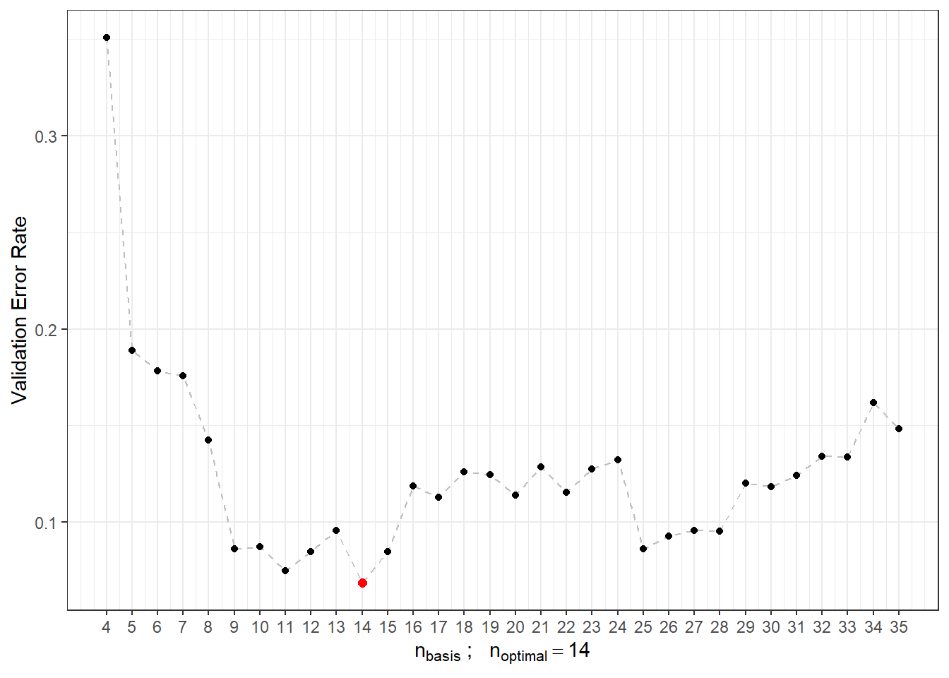
Figure 1.15: Dependence of validation error on the value of \(n_{basis}\), i.e., on the number of bases.
We can now define the final model using functional logistic regression, choosing the B-spline basis for \(\beta(t)\) with 14 bases.
Code
# optimal model
basis2 <- create.bspline.basis(rangeval = range(tt), nbasis = n.basis.opt)
f <- Y ~ x
# bases for x and betas
basis.x <- list("x" = basis1)
basis.b <- list("x" = basis2)
# input data for the model
dataf <- as.data.frame(y.train)
colnames(dataf) <- "Y"
ldata <- list("df" = dataf, "x" = x.train)
# binomial model ... logistic regression model
model.glm <- fregre.glm(f, family = binomial(), data = ldata,
basis.x = basis.x, basis.b = basis.b)
# accuracy on training data
predictions.train <- predict(model.glm, newx = ldata)
predictions.train <- data.frame(Y.pred = ifelse(predictions.train < 1/2, 0, 1))
presnost.train <- table(Y.train, predictions.train$Y.pred) |>
prop.table() |> diag() |> sum()
# accuracy on test data
newldata = list("df" = as.data.frame(Y.test), "x" = fdata(X.test))
predictions.test <- predict(model.glm, newx = newldata)
predictions.test <- data.frame(Y.pred = ifelse(predictions.test < 1/2, 0, 1))
presnost.test <- table(Y.test, predictions.test$Y.pred) |>
prop.table() |> diag() |> sum()We have calculated the training error rate (which is 5 %) and the test error rate (which is 11.67 %). For better visualization, we can also plot the estimated probabilities of belonging to the classification class \(Y = 1\) on the training data against the values of the linear predictor.
Code
data.frame(
linear.predictor = model.glm$linear.predictors,
response = model.glm$fitted.values,
Y = factor(y.train)
) |> ggplot(aes(x = linear.predictor, y = response, colour = Y)) +
geom_point(size = 1.5) +
scale_colour_discrete(labels = c('Y = 0', 'Y = 1')) +
geom_abline(aes(slope = 0, intercept = 0.5), linetype = 'dashed') +
theme_bw() +
labs(x = 'Linear Predictor',
y = 'Estimated Probability Pr(Y = 1|X = x)',
colour = 'Class') 
Figure 5.5: Dependence of estimated probabilities on the values of the linear predictor. Points are color-coded according to their classification class.
For informational purposes, we can also display the progression of the estimated parametric function \(\beta(t)\).
Code
t.seq <- seq(0, 6, length = 1001)
beta.seq <- eval.fd(evalarg = t.seq, fdobj = model.glm$beta.l$x)
data.frame(t = t.seq, beta = beta.seq) |>
ggplot(aes(t, beta)) +
geom_line() +
theme_bw() +
labs(x = 'Time',
y = expression(widehat(beta)(t))) +
theme(panel.grid.major = element_blank(), panel.grid.minor = element_blank()) +
geom_abline(aes(slope = 0, intercept = 0), linetype = 'dashed',
linewidth = 0.5, colour = 'grey')![Plot of the estimated parametric function $\beta(t), t \in [0, 6]$.](05-Simulace_deriv2_files/figure-html/unnamed-chunk-49-1.png)
Figure 5.6: Plot of the estimated parametric function \(\beta(t), t \in [0, 6]\).
Finally, we will add the results to the summary table.
5.1.3.4.2 Logistic Regression with Principal Component Analysis
To construct this classifier, we need to perform functional principal component analysis, determine the appropriate number of components, and calculate the score values for the test data. We have already completed this in the linear discriminant analysis section, so we will use these results in the following section.
We can directly construct the logistic regression model using the glm(, family = binomial) function.
Code
# model
clf.LR <- glm(Y ~ ., data = data.PCA.train, family = binomial)
# accuracy on training data
predictions.train <- predict(clf.LR, newdata = data.PCA.train, type = 'response')
predictions.train <- ifelse(predictions.train > 0.5, 1, 0)
presnost.train <- table(data.PCA.train$Y, predictions.train) |>
prop.table() |> diag() |> sum()
# accuracy on test data
predictions.test <- predict(clf.LR, newdata = data.PCA.test, type = 'response')
predictions.test <- ifelse(predictions.test > 0.5, 1, 0)
presnost.test <- table(data.PCA.test$Y, predictions.test) |>
prop.table() |> diag() |> sum()We have calculated the error rate of the classifier on the training data (31.43 %) and on the test data (23.33 %).
For graphical representation of the method, we can plot the decision boundary in the scores of the first two principal components. We will compute this boundary on a dense grid of points and display it using the geom_contour() function, just as we did in the LDA and QDA cases.
Code
nd <- nd |> mutate(prd = as.numeric(predict(clf.LR, newdata = nd,
type = 'response')))
nd$prd <- ifelse(nd$prd > 0.5, 1, 0)
data.PCA.train |> ggplot(aes(x = V1, y = V2, colour = Y)) +
geom_point(size = 1.5) +
labs(x = paste('1st Principal Component (explained variance',
round(100 * data.PCA$varprop[1], 2), '%)'),
y = paste('2nd Principal Component (',
round(100 * data.PCA$varprop[2], 2), '%)'),
colour = 'Group') +
scale_colour_discrete(labels = c('Y = 0', 'Y = 1')) +
theme_bw() +
geom_contour(data = nd, aes(x = V1, y = V2, z = prd), colour = 'black')
Figure 5.7: Scores of the first two principal components, color-coded according to classification class. The decision boundary (a line in the plane of the first two principal components) between classes is indicated in black, constructed using logistic regression.
Note that the decision boundary between the classification classes is now a line, similar to the case with LDA.
Finally, we will add the error rates to the summary table.
5.1.3.5 Decision Trees
In this section, we will look at a very different approach to constructing a classifier compared to methods such as LDA or logistic regression. Decision trees are a very popular tool for classification; however, like some of the previous methods, they are not directly designed for functional data. There are, however, procedures to convert functional objects into multidimensional ones, allowing us to apply decision tree algorithms. We can consider the following approaches:
An algorithm built on basis coefficients,
Utilizing principal component scores,
Discretizing the interval and evaluating the function only on a finite grid of points.
We will first focus on discretizing the interval and then compare the results with the other two approaches to constructing decision trees.
5.1.3.5.1 Interval Discretization
First, we need to define points from the interval \(I = [0, 6]\), where we will evaluate the functions. Next, we will create an object where the rows represent the individual (discretized) functions and the columns represent time. Finally, we will add a column \(Y\) containing information about the classification class and repeat the same for the test data.
Code
# sequence of points at which we will evaluate the functions
t.seq <- seq(0, 6, length = 101)
grid.data <- eval.fd(fdobj = X.train, evalarg = t.seq)
grid.data <- as.data.frame(t(grid.data)) # transpose for functions in rows
grid.data$Y <- Y.train |> factor()
grid.data.test <- eval.fd(fdobj = X.test, evalarg = t.seq)
grid.data.test <- as.data.frame(t(grid.data.test))
grid.data.test$Y <- Y.test |> factor()Now we can construct a decision tree where all times from the vector t.seq will serve as predictors. This classification method is not susceptible to multicollinearity, so we do not need to worry about it. We will choose accuracy as the metric.
Code
# model construction
clf.tree <- train(Y ~ ., data = grid.data,
method = "rpart",
trControl = trainControl(method = "CV", number = 10),
metric = "Accuracy")
# accuracy on training data
predictions.train <- predict(clf.tree, newdata = grid.data)
presnost.train <- table(Y.train, predictions.train) |>
prop.table() |> diag() |> sum()
# accuracy on test data
predictions.test <- predict(clf.tree, newdata = grid.data.test)
presnost.test <- table(Y.test, predictions.test) |>
prop.table() |> diag() |> sum()The error rate of the classifier on the test data is thus 18.33 %, and on the training data 26.43 %.
We can visualize the decision tree graphically using the fancyRpartPlot() function. We will set the colors of the nodes to reflect the previous color differentiation. This is an unpruned tree.
Code
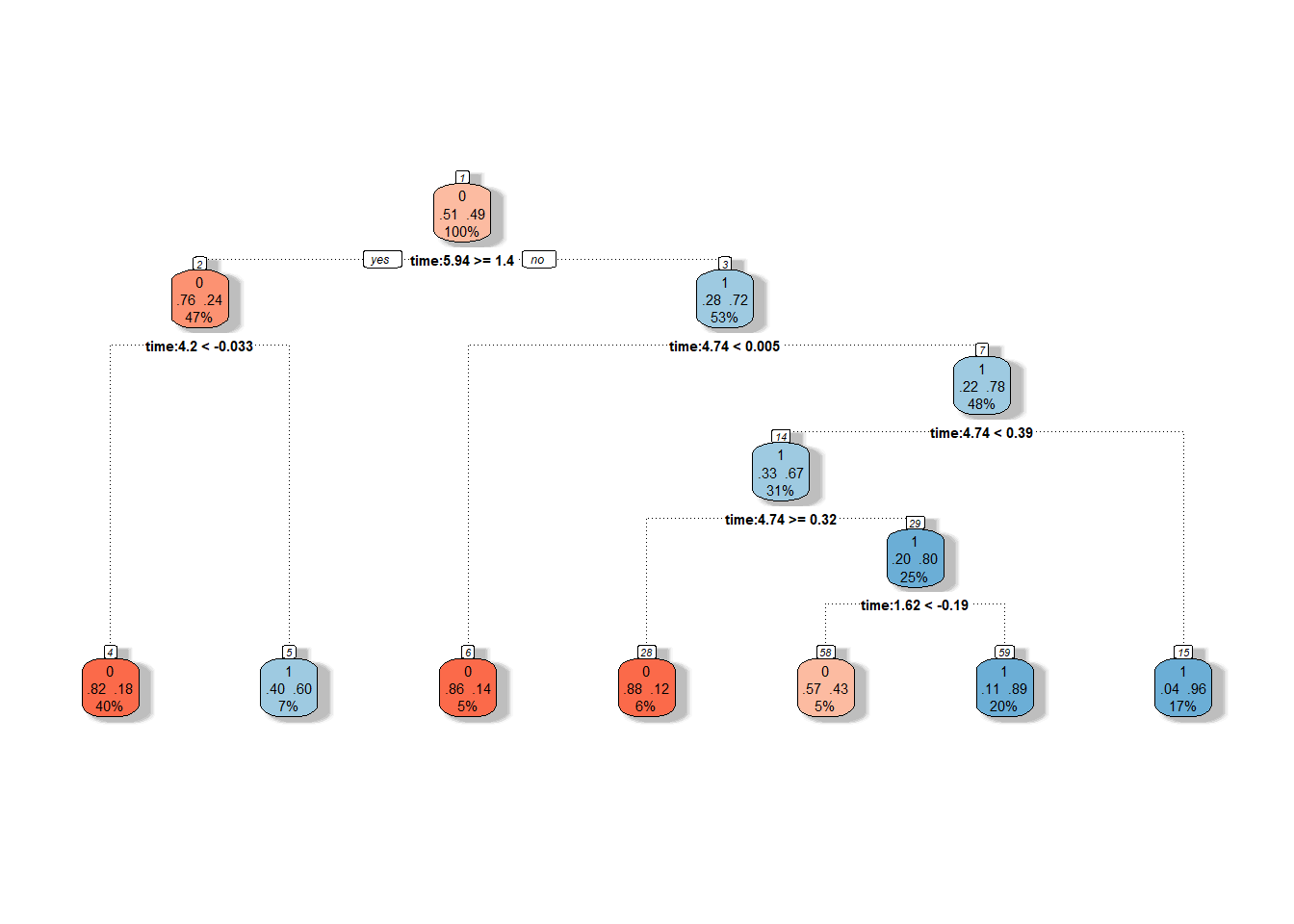
Figure 1.18: Graphical representation of the unpruned decision tree. Blue shades represent nodes belonging to classification class 1, and red shades represent class 0.
We can also plot the final pruned decision tree.
Code
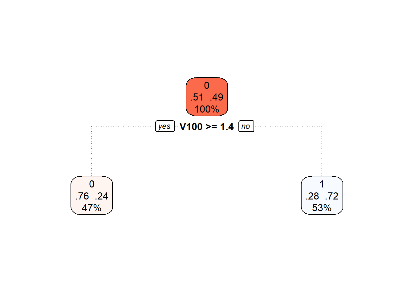
Figure 5.8: Final pruned decision tree.
Finally, we will again add the training and test error rates to the summary table.
5.1.3.5.2 Principal Component Scores
Another option for constructing a decision tree is to use principal component scores. Since we have already calculated the scores for the previous classification methods, we will utilize this knowledge and construct a decision tree based on the scores of the first 3 principal components.
Code
# model construction
clf.tree.PCA <- train(Y ~ ., data = data.PCA.train,
method = "rpart",
trControl = trainControl(method = "CV", number = 10),
metric = "Accuracy")
# accuracy on training data
predictions.train <- predict(clf.tree.PCA, newdata = data.PCA.train)
presnost.train <- table(Y.train, predictions.train) |>
prop.table() |> diag() |> sum()
# accuracy on test data
predictions.test <- predict(clf.tree.PCA, newdata = data.PCA.test)
presnost.test <- table(Y.test, predictions.test) |>
prop.table() |> diag() |> sum()The error rate of the decision tree on the test data is thus 23.33 %, and on the training data 30 %.
We can visualize the decision tree constructed on the principal component scores using the fancyRpartPlot() function. We will set the colors of the nodes to reflect the previous color differentiation. This is an unpruned tree.
Code
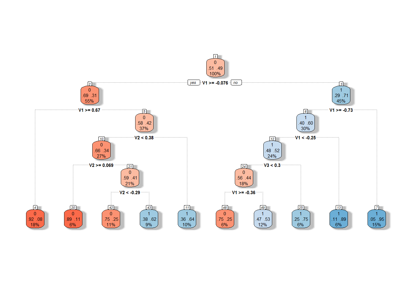
Figure 1.20: Graphical representation of the unpruned decision tree constructed on principal component scores. Blue shades represent nodes belonging to classification class 1, and red shades represent class 0.
We can also plot the final pruned decision tree.
Code
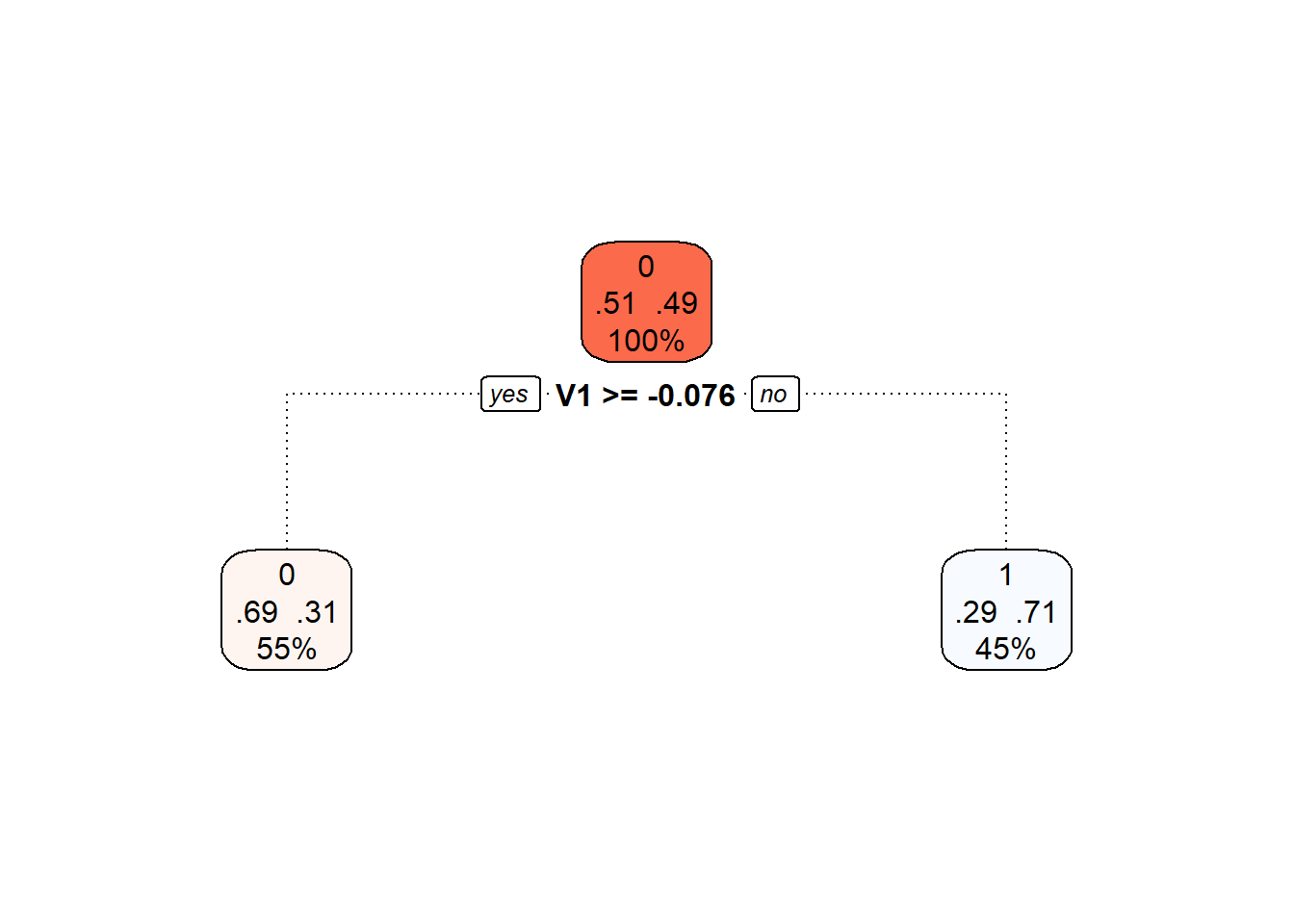
Figure 3.1: Final pruned decision tree.
Finally, we will again add the training and test error rates to the summary table.
5.1.3.5.3 Basis Coefficients
The final option we will utilize for constructing a decision tree is to use coefficients in the representation of functions in the B-spline basis.
First, let’s define the necessary datasets with the coefficients.
Code
Now we can construct the classifier.
Code
# model construction
clf.tree.Bbasis <- train(Y ~ ., data = data.Bbasis.train,
method = "rpart",
trControl = trainControl(method = "CV", number = 10),
metric = "Accuracy")
# accuracy on training data
predictions.train <- predict(clf.tree.Bbasis, newdata = data.Bbasis.train)
presnost.train <- table(Y.train, predictions.train) |>
prop.table() |> diag() |> sum()
# accuracy on test data
predictions.test <- predict(clf.tree.Bbasis, newdata = data.Bbasis.test)
presnost.test <- table(Y.test, predictions.test) |>
prop.table() |> diag() |> sum()The error rate of the decision tree on the training data is thus 26.43 %, and on the test data 18.33 %.
We can visualize the decision tree constructed on the B-spline coefficient representation using the fancyRpartPlot() function. We will set the colors of the nodes to reflect the previous color differentiation. This is an unpruned tree.
Code
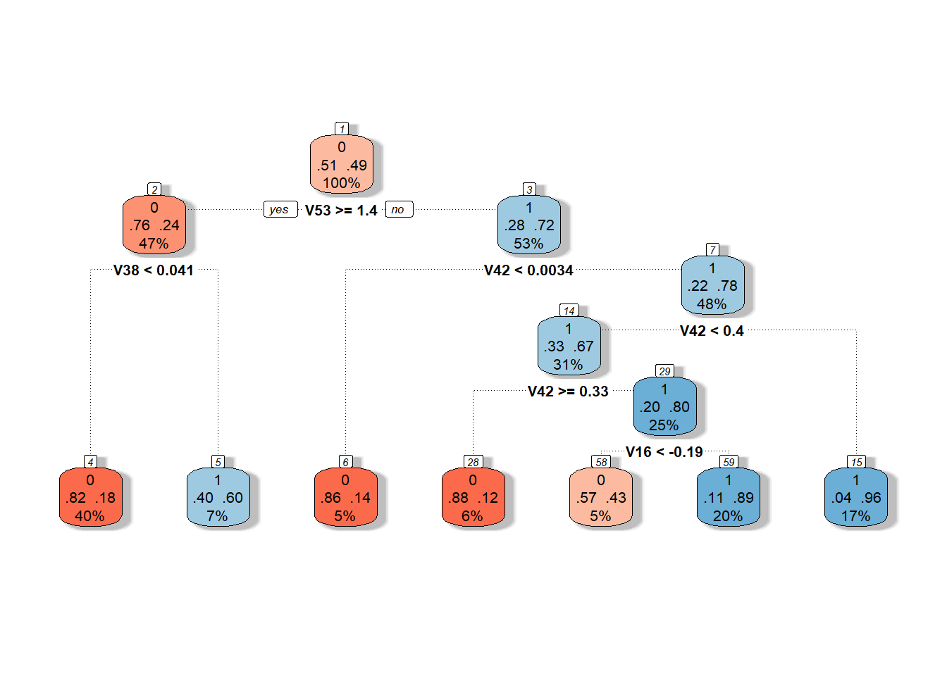
Figure 1.22: Graphical representation of the unpruned decision tree constructed on basis coefficients. Blue shades represent nodes belonging to classification class 1, and red shades represent class 0.
We can also plot the final pruned decision tree.
Code
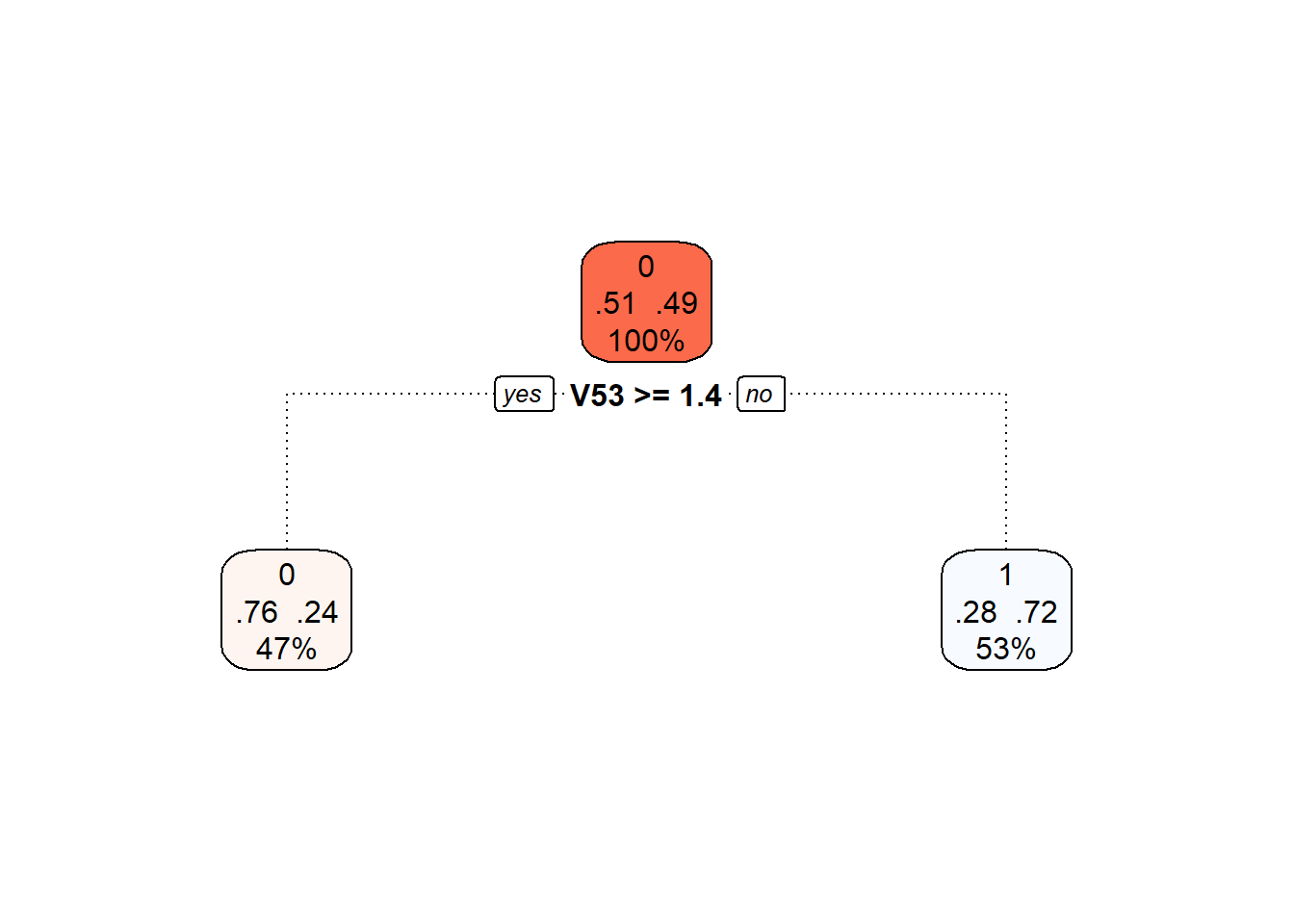
Figure 5.9: Final pruned decision tree.
Finally, we will again add the training and test error rates to the summary table.
5.1.3.6 Random Forests
The classifier constructed using the random forests method consists of building several individual decision trees, which are then combined to create a common classifier (via “voting”).
As with decision trees, we have several options regarding which data (finite-dimensional) we will use to construct the model. We will again consider the three approaches discussed above. The datasets with the corresponding variables for all three approaches have already been prepared from the previous section, so we can directly construct the models, calculate the characteristics of the classifiers, and add the results to the summary table.
5.1.3.6.1 Interval Discretization
In the first case, we utilize the evaluation of functions on a given grid of points over the interval \(I = [0, 6]\).
Code
# model construction
clf.RF <- randomForest(Y ~ ., data = grid.data,
ntree = 500, # number of trees
importance = TRUE,
nodesize = 5)
# accuracy on training data
predictions.train <- predict(clf.RF, newdata = grid.data)
presnost.train <- table(Y.train, predictions.train) |>
prop.table() |> diag() |> sum()
# accuracy on test data
predictions.test <- predict(clf.RF, newdata = grid.data.test)
presnost.test <- table(Y.test, predictions.test) |>
prop.table() |> diag() |> sum()The error rate of the random forest on the training data is thus 0 %, and on the test data 20 %.
5.1.3.6.2 Principal Component Scores
In this case, we will use the scores of the first $p = $ 3 principal components.
Code
# model construction
clf.RF.PCA <- randomForest(Y ~ ., data = data.PCA.train,
ntree = 500, # number of trees
importance = TRUE,
nodesize = 5)
# accuracy on training data
predictions.train <- predict(clf.RF.PCA, newdata = data.PCA.train)
presnost.train <- table(Y.train, predictions.train) |>
prop.table() |> diag() |> sum()
# accuracy on test data
predictions.test <- predict(clf.RF.PCA, newdata = data.PCA.test)
presnost.test <- table(Y.test, predictions.test) |>
prop.table() |> diag() |> sum()The error rate on the training data is thus 1.43 %, and on the test data 30 %.
5.1.3.6.3 Basis Coefficients
Finally, we will use the representation of functions through the B-spline basis.
Code
# model construction
clf.RF.Bbasis <- randomForest(Y ~ ., data = data.Bbasis.train,
ntree = 500, # number of trees
importance = TRUE,
nodesize = 5)
# accuracy on training data
predictions.train <- predict(clf.RF.Bbasis, newdata = data.Bbasis.train)
presnost.train <- table(Y.train, predictions.train) |>
prop.table() |> diag() |> sum()
# accuracy on test data
predictions.test <- predict(clf.RF.Bbasis, newdata = data.Bbasis.test)
presnost.test <- table(Y.test, predictions.test) |>
prop.table() |> diag() |> sum()The error rate of this classifier on the training data is 0 %, and on the test data 18.33 %.
5.1.3.7 Support Vector Machines
Now let’s look at classifying our simulated curves using the Support Vector Machines (SVM) method. The advantage of this classification method is its computational efficiency, as it defines the boundary curve between classes using only a few (often very few) observations.
In the case of functional data, we have several options for applying the SVM method. The simplest variant is to use this classification method directly on the discretized function (section 5.1.3.7.2). Another option is to utilize the principal component scores to classify curves based on their representation 5.1.3.7.3. A straightforward variant is to use the representation of curves through the B-spline basis and classify curves based on the coefficients of their representation in this basis (section 5.1.3.7.4).
A more complex consideration can lead us to several additional options that leverage the functional nature of the data. We can utilize projections of functions onto a subspace generated, for example, by B-spline functions (section 5.1.3.7.5). The final method we will use for classifying functional data involves combining projection onto a certain subspace generated by functions (Reproducing Kernel Hilbert Space, RKHS) and classifying the corresponding representation. This method utilizes not only the classical SVM but also SVM for regression, as discussed in section RKHS + SVM 5.1.3.7.6.
5.1.3.7.1 SVM for Functional Data
In the fda.usc library, we will use the function classif.svm() to apply the SVM method directly to functional data. First, we will create suitable objects for constructing the classifier.
Code
# set norm equal to one
norms <- c()
for (i in 1:dim(XXder$coefs)[2]) {
norms <- c(norms, as.numeric(1 / norm.fd(XXder[i])))
}
XXfd_norm <- XXder
XXfd_norm$coefs <- XXfd_norm$coefs * matrix(norms,
ncol = dim(XXder$coefs)[2],
nrow = dim(XXder$coefs)[1],
byrow = TRUE)
# split into test and training sets
X.train_norm <- subset(XXfd_norm, split == TRUE)
X.test_norm <- subset(XXfd_norm, split == FALSE)
Y.train_norm <- subset(Y, split == TRUE)
Y.test_norm <- subset(Y, split == FALSE)
grid.data <- eval.fd(fdobj = X.train_norm, evalarg = t.seq)
grid.data <- as.data.frame(t(grid.data))
grid.data$Y <- Y.train_norm |> factor()
grid.data.test <- eval.fd(fdobj = X.test_norm, evalarg = t.seq)
grid.data.test <- as.data.frame(t(grid.data.test))
grid.data.test$Y <- Y.test_norm |> factor()Code
Finally, we can construct the classifiers on the entire training data with the hyperparameter values (determined previously by CV). We will also determine the errors on the test and training data.
Code
# Create suitable objects
x.train <- fdata(X.train_norm)
y.train <- as.factor(Y.train_norm)
# Points at which the functions are evaluated
tt <- x.train[["argvals"]]
dataf <- as.data.frame(y.train)
colnames(dataf) <- "Y"
# B-spline basis
basis1 <- X.train_norm$basis
# Formula
f <- Y ~ x
# Basis for x
basis.x <- list("x" = basis1)
# Input data for the model
ldata <- list("df" = dataf, "x" = x.train)Code
## Warning in Minverse(t(B) %*% B): System is computationally singular (rank 54)
##
## The matrix inverse is computed by svd (effective rank 52)Code
## Warning in Minverse(t(B) %*% B): System is computationally singular (rank 54)
##
## The matrix inverse is computed by svd (effective rank 52)Code
## Warning in Minverse(t(B) %*% B): System is computationally singular (rank 54)
##
## The matrix inverse is computed by svd (effective rank 52)Code
# Accuracy on training data
newdat <- list("x" = x.train)
predictions.train.l <- predict(model.svm.f_l, newdat, type = 'class')
accuracy.train.l <- mean(factor(Y.train_norm) == predictions.train.l)
predictions.train.p <- predict(model.svm.f_p, newdat, type = 'class')
accuracy.train.p <- mean(factor(Y.train_norm) == predictions.train.p)
predictions.train.r <- predict(model.svm.f_r, newdat, type = 'class')
accuracy.train.r <- mean(factor(Y.train_norm) == predictions.train.r)
# Accuracy on test data
newdat <- list("x" = fdata(X.test_norm))
predictions.test.l <- predict(model.svm.f_l, newdat, type = 'class')
accuracy.test.l <- mean(factor(Y.test_norm) == predictions.test.l)
predictions.test.p <- predict(model.svm.f_p, newdat, type = 'class')
accuracy.test.p <- mean(factor(Y.test_norm) == predictions.test.p)
predictions.test.r <- predict(model.svm.f_r, newdat, type = 'class')
accuracy.test.r <- mean(factor(Y.test_norm) == predictions.test.r)The error rate of the SVM method on the training data is thus 15.7143 % for the linear kernel, 12.1429 % for the polynomial kernel, and 15.7143 % for the Gaussian kernel. On the test data, the error rate of the method is 16.6667 % for the linear kernel, 25 % for the polynomial kernel, and 23.3333 % for the radial kernel.
5.1.3.7.2 Interval Discretization
Let’s continue by applying the Support Vector Machines method directly to the discretized data (evaluation of the function on a grid of points over the interval \(I = [0, 6]\)), considering all three aforementioned kernel functions.
We will now classify the normalized data using the classic SVM method, selecting parameters as follows. For one generated dataset, we will determine parameters using cross-validation (CV), and these parameters will then be applied to other simulated data.
Code
# model construction
clf.SVM.l <- svm(Y ~ ., data = grid.data,
type = 'C-classification',
scale = TRUE,
cost = 25,
kernel = 'linear')
clf.SVM.p <- svm(Y ~ ., data = grid.data,
type = 'C-classification',
scale = TRUE,
coef0 = 1,
cost = 0.7,
kernel = 'polynomial')
clf.SVM.r <- svm(Y ~ ., data = grid.data,
type = 'C-classification',
scale = TRUE,
cost = 55,
gamma = 0.0005,
kernel = 'radial')
# accuracy on training data
predictions.train.l <- predict(clf.SVM.l, newdata = grid.data)
presnost.train.l <- table(Y.train, predictions.train.l) |>
prop.table() |> diag() |> sum()
predictions.train.p <- predict(clf.SVM.p, newdata = grid.data)
presnost.train.p <- table(Y.train, predictions.train.p) |>
prop.table() |> diag() |> sum()
predictions.train.r <- predict(clf.SVM.r, newdata = grid.data)
presnost.train.r <- table(Y.train, predictions.train.r) |>
prop.table() |> diag() |> sum()
# accuracy on test data
predictions.test.l <- predict(clf.SVM.l, newdata = grid.data.test)
presnost.test.l <- table(Y.test, predictions.test.l) |>
prop.table() |> diag() |> sum()
predictions.test.p <- predict(clf.SVM.p, newdata = grid.data.test)
presnost.test.p <- table(Y.test, predictions.test.p) |>
prop.table() |> diag() |> sum()
predictions.test.r <- predict(clf.SVM.r, newdata = grid.data.test)
presnost.test.r <- table(Y.test, predictions.test.r) |>
prop.table() |> diag() |> sum()The error rate of the SVM method on the training data is thus 7.86 % for the linear kernel, 12.86 % for the polynomial kernel, and 14.29 % for the Gaussian kernel. On the test data, the error rates are 10 % for the linear kernel, 23.33 % for the polynomial kernel, and 23.33 % for the radial kernel.
5.1.3.7.3 Principal Component Scores
In this case, we will use the scores of the first \(p =\) 3 principal components.
Code
# model construction
clf.SVM.l.PCA <- svm(Y ~ ., data = data.PCA.train,
type = 'C-classification',
scale = TRUE,
cost = 0.1,
kernel = 'linear')
clf.SVM.p.PCA <- svm(Y ~ ., data = data.PCA.train,
type = 'C-classification',
scale = TRUE,
coef0 = 1,
cost = 0.01,
kernel = 'polynomial')
clf.SVM.r.PCA <- svm(Y ~ ., data = data.PCA.train,
type = 'C-classification',
scale = TRUE,
cost = 1,
gamma = 0.01,
kernel = 'radial')
# accuracy on training data
predictions.train.l <- predict(clf.SVM.l.PCA, newdata = data.PCA.train)
accuracy.train.l <- table(data.PCA.train$Y, predictions.train.l) |>
prop.table() |> diag() |> sum()
predictions.train.p <- predict(clf.SVM.p.PCA, newdata = data.PCA.train)
accuracy.train.p <- table(data.PCA.train$Y, predictions.train.p) |>
prop.table() |> diag() |> sum()
predictions.train.r <- predict(clf.SVM.r.PCA, newdata = data.PCA.train)
accuracy.train.r <- table(data.PCA.train$Y, predictions.train.r) |>
prop.table() |> diag() |> sum()
# accuracy on test data
predictions.test.l <- predict(clf.SVM.l.PCA, newdata = data.PCA.test)
accuracy.test.l <- table(data.PCA.test$Y, predictions.test.l) |>
prop.table() |> diag() |> sum()
predictions.test.p <- predict(clf.SVM.p.PCA, newdata = data.PCA.test)
accuracy.test.p <- table(data.PCA.test$Y, predictions.test.p) |>
prop.table() |> diag() |> sum()
predictions.test.r <- predict(clf.SVM.r.PCA, newdata = data.PCA.test)
accuracy.test.r <- table(data.PCA.test$Y, predictions.test.r) |>
prop.table() |> diag() |> sum()The error rate of the SVM method applied to the principal component scores on the training data is therefore 31.43 % for the linear kernel, 31.43 % for the polynomial kernel, and 32.14 % for the Gaussian kernel. On the test data, the error rate is then 23.33 % for the linear kernel, 23.33 % for the polynomial kernel, and 23.33 % for the radial kernel.
To graphically illustrate the method, we can mark the decision boundary on the graph of the scores of the first two principal components. We will calculate this boundary on a dense grid of points and display it using the geom_contour() function, just as we did in previous cases when plotting the classification boundary.
Code
nd <- rbind(nd, nd, nd) |> mutate(
prd = c(as.numeric(predict(clf.SVM.l.PCA, newdata = nd, type = 'response')),
as.numeric(predict(clf.SVM.p.PCA, newdata = nd, type = 'response')),
as.numeric(predict(clf.SVM.r.PCA, newdata = nd, type = 'response'))),
kernel = rep(c('linear', 'polynomial', 'radial'),
each = length(as.numeric(predict(clf.SVM.l.PCA,
newdata = nd,
type = 'response')))))
data.PCA.train |> ggplot(aes(x = V1, y = V2, colour = Y)) +
geom_point(size = 1.5) +
labs(x = paste('1st principal component (explained variance',
round(100 * data.PCA$varprop[1], 2), '%)'),
y = paste('2nd principal component (',
round(100 * data.PCA$varprop[2], 2), '%)'),
colour = 'Group',
linetype = 'Kernel type') +
scale_colour_discrete(labels = c('Y = 0', 'Y = 1')) +
theme_bw() +
geom_contour(data = nd, aes(x = V1, y = V2, z = prd, linetype = kernel),
colour = 'black') +
geom_contour(data = nd, aes(x = V1, y = V2, z = prd, linetype = kernel),
colour = 'black') +
geom_contour(data = nd, aes(x = V1, y = V2, z = prd, linetype = kernel),
colour = 'black')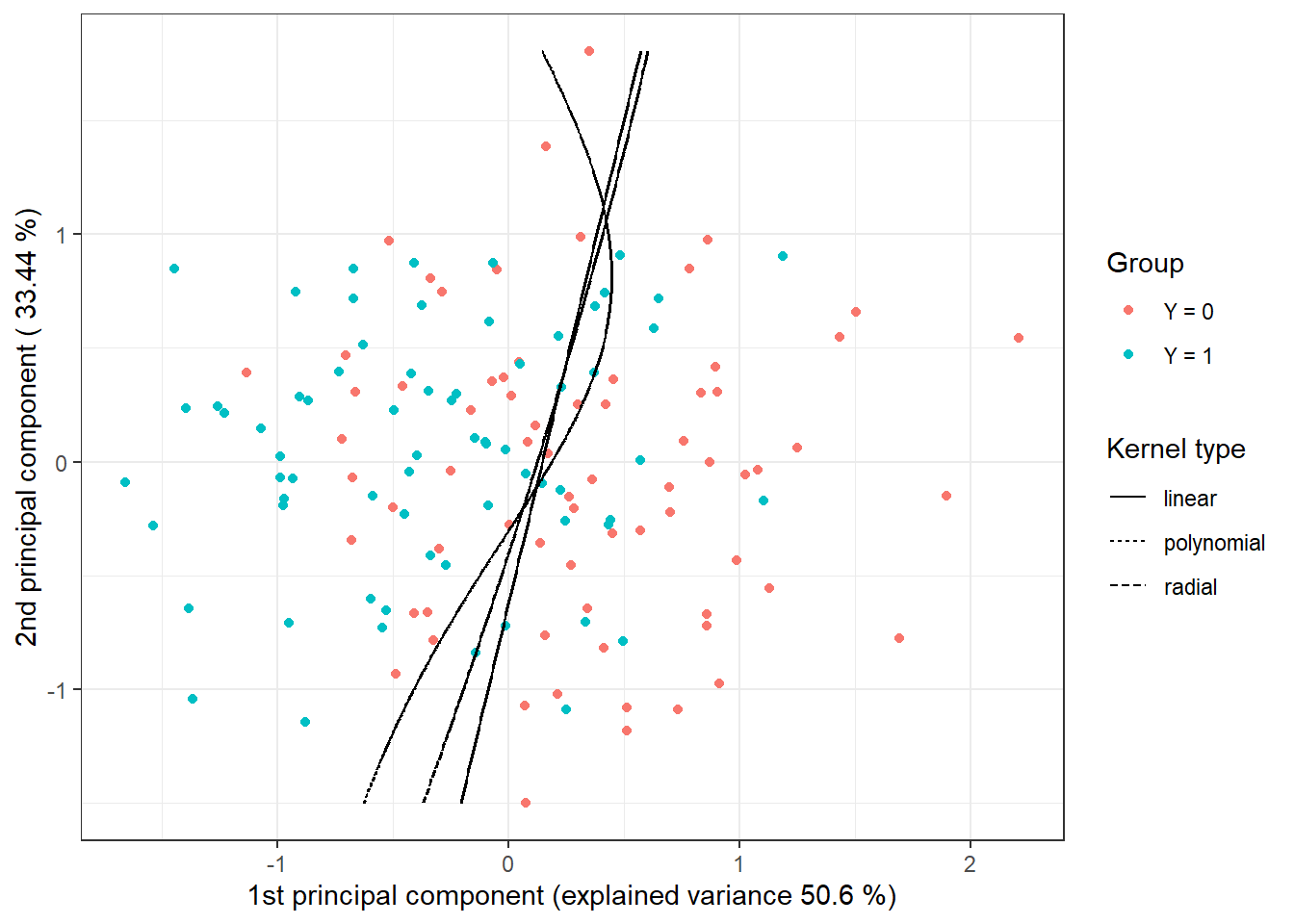
Figure 5.10: Scores of the first two principal components, color-coded according to classification group membership. The decision boundary (line or curves in the plane of the first two principal components) between classes constructed using the SVM method is highlighted in black.
5.1.3.7.4 B-spline Coefficients
Finally, we will use function representations through the B-spline basis.
Code
# Building the model
clf.SVM.l.Bbasis <- svm(Y ~ ., data = data.Bbasis.train,
type = 'C-classification',
scale = TRUE,
cost = 50,
kernel = 'linear')
clf.SVM.p.Bbasis <- svm(Y ~ ., data = data.Bbasis.train,
type = 'C-classification',
scale = TRUE,
coef0 = 1,
cost = 0.1,
kernel = 'polynomial')
clf.SVM.r.Bbasis <- svm(Y ~ ., data = data.Bbasis.train,
type = 'C-classification',
scale = TRUE,
cost = 100,
gamma = 0.001,
kernel = 'radial')
# Accuracy on training data
predictions.train.l <- predict(clf.SVM.l.Bbasis, newdata = data.Bbasis.train)
accuracy.train.l <- table(Y.train, predictions.train.l) |>
prop.table() |> diag() |> sum()
predictions.train.p <- predict(clf.SVM.p.Bbasis, newdata = data.Bbasis.train)
accuracy.train.p <- table(Y.train, predictions.train.p) |>
prop.table() |> diag() |> sum()
predictions.train.r <- predict(clf.SVM.r.Bbasis, newdata = data.Bbasis.train)
accuracy.train.r <- table(Y.train, predictions.train.r) |>
prop.table() |> diag() |> sum()
# Accuracy on test data
predictions.test.l <- predict(clf.SVM.l.Bbasis, newdata = data.Bbasis.test)
accuracy.test.l <- table(Y.test, predictions.test.l) |>
prop.table() |> diag() |> sum()
predictions.test.p <- predict(clf.SVM.p.Bbasis, newdata = data.Bbasis.test)
accuracy.test.p <- table(Y.test, predictions.test.p) |>
prop.table() |> diag() |> sum()
predictions.test.r <- predict(clf.SVM.r.Bbasis, newdata = data.Bbasis.test)
accuracy.test.r <- table(Y.test, predictions.test.r) |>
prop.table() |> diag() |> sum()The error rate of the SVM method applied to the B-spline coefficients on the training data is therefore 7.14 % for the linear kernel, 20 % for the polynomial kernel, and 12.86 % for the Gaussian kernel. On the test data, the error rate of the method is 6.67 % for the linear kernel, 21.67 % for the polynomial kernel, and 20 % for the radial kernel.
5.1.3.7.5 Projection onto B-spline Basis
Another option for using the classical SVM method for functional data is to project the original data onto some \(d\)-dimensional subspace of our Hilbert space \(\mathcal{H}\), denoted as \(V_d\). Assume that this subspace \(V_d\) has an orthonormal basis \(\{\Psi_j\}_{j = 1, \dots, d}\). We define the transformation \(P_{V_d}\) as the orthogonal projection onto the subspace \(V_d\), so we can write:
\[ P_{V_d} (x) = \sum_{j = 1}^d \langle x, \Psi_j \rangle \Psi_j. \]
Now we can use the coefficients from the orthogonal projection for classification, that is, we apply the standard SVM to the vectors \(\left( \langle x, \Psi_1 \rangle, \dots, \langle x, \Psi_d \rangle\right)^\top\). By using this transformation, we have defined a new so-called adapted kernel, which consists of the orthogonal projection \(P_{V_d}\) and the kernel function of the standard support vector method. Thus, we have (adapted) kernel \(Q(x_i, x_j) = K(P_{V_d}(x_i), P_{V_d}(x_j))\). This is a dimensionality reduction method, which we can call filtering.
For the projection itself, we will use the project.basis() function from the fda library in R. Its input will be a matrix of the original discrete (non-smoothed) data, the values at which we measure values in the original data matrix, and the basis object onto which we want to project the data. We will choose projection onto a B-spline basis since the use of a Fourier basis is not suitable for our non-periodic data.
We choose the dimension \(d\) either from some prior expert knowledge or by using cross-validation. In our case, we will determine the optimal dimension of the subspace \(V_d\) using \(k\)-fold cross-validation (we choose \(k \ll n\) due to the computational intensity of the method, often \(k = 5\) or \(k = 10\)). We require B-splines of order 4, for which the relationship for the number of basis functions holds:
\[ n_{basis} = n_{breaks} + n_{order} - 2, \]
where \(n_{breaks}\) is the number of knots and \(n_{order} = 4\). Therefore, the minimum dimension (for \(n_{breaks} = 1\)) is chosen as \(n_{basis} = 3\), and the maximum (for \(n_{breaks} = 51\), corresponding to the number of original discrete data points) is \(n_{basis} = 53\). However, in R, the value of \(n_{basis}\) must be at least \(n_{order} = 4\), and for large values of \(n_{basis}\), we already experience model overfitting; therefore, we choose a maximum \(n_{basis}\) of a smaller number, say 43.
Code
k_cv <- 10 # k-fold CV
# Values for B-spline basis
rangeval <- range(t)
norder <- 4
n_basis_min <- norder
n_basis_max <- length(t) + norder - 2 - 10
dimensions <- n_basis_min:n_basis_max # all dimensions we want to try
# Split the training data into k parts
folds <- createMultiFolds(1:sum(split), k = k_cv, time = 1)
# List with three components ... matrices for individual kernels -> linear, poly, radial
# An empty matrix where we will insert individual results
# Columns will contain accuracy values for each part of the training set
# Rows will contain values for each dimension value
CV.results <- list(SVM.l = matrix(NA, nrow = length(dimensions), ncol = k_cv),
SVM.p = matrix(NA, nrow = length(dimensions), ncol = k_cv),
SVM.r = matrix(NA, nrow = length(dimensions), ncol = k_cv))
for (d in dimensions) {
# Basis object
bbasis <- create.bspline.basis(rangeval = rangeval,
nbasis = d)
# Projection of discrete data onto the B-spline basis of dimension d
Projection <- project.basis(y = grid.data |> select(!contains('Y')) |> as.matrix() |> t(), # matrix of discrete data
argvals = t.seq, # vector of arguments
basisobj = bbasis) # basis object
# Splitting into training and test data within CV
XX.train <- t(Projection) # subset(t(Projection), split == TRUE)
for (index_cv in 1:k_cv) {
# Definition of test and training parts for CV
fold <- folds[[index_cv]]
cv_sample <- 1:dim(XX.train)[1] %in% fold
data.projection.train.cv <- as.data.frame(XX.train[cv_sample, ])
data.projection.train.cv$Y <- factor(Y.train[cv_sample])
data.projection.test.cv <- as.data.frame(XX.train[!cv_sample, ])
Y.test.cv <- Y.train[!cv_sample]
data.projection.test.cv$Y <- factor(Y.test.cv)
# Building the models
clf.SVM.l.projection <- svm(Y ~ ., data = data.projection.train.cv,
type = 'C-classification',
scale = TRUE,
kernel = 'linear')
clf.SVM.p.projection <- svm(Y ~ ., data = data.projection.train.cv,
type = 'C-classification',
scale = TRUE,
coef0 = 1,
kernel = 'polynomial')
clf.SVM.r.projection <- svm(Y ~ ., data = data.projection.train.cv,
type = 'C-classification',
scale = TRUE,
kernel = 'radial')
# Accuracy on validation data
## linear kernel
predictions.test.l <- predict(clf.SVM.l.projection,
newdata = data.projection.test.cv)
accuracy.test.l <- table(Y.test.cv, predictions.test.l) |>
prop.table() |> diag() |> sum()
## polynomial kernel
predictions.test.p <- predict(clf.SVM.p.projection,
newdata = data.projection.test.cv)
accuracy.test.p <- table(Y.test.cv, predictions.test.p) |>
prop.table() |> diag() |> sum()
## radial kernel
predictions.test.r <- predict(clf.SVM.r.projection,
newdata = data.projection.test.cv)
accuracy.test.r <- table(Y.test.cv, predictions.test.r) |>
prop.table() |> diag() |> sum()
# Insert accuracies into positions for given d and fold
CV.results$SVM.l[d - min(dimensions) + 1, index_cv] <- accuracy.test.l
CV.results$SVM.p[d - min(dimensions) + 1, index_cv] <- accuracy.test.p
CV.results$SVM.r[d - min(dimensions) + 1, index_cv] <- accuracy.test.r
}
}
# Compute average accuracies for individual d across folds
for (n_method in 1:length(CV.results)) {
CV.results[[n_method]] <- apply(CV.results[[n_method]], 1, mean)
}
d.opt <- c(which.max(CV.results$SVM.l) + n_basis_min - 1,
which.max(CV.results$SVM.p) + n_basis_min - 1,
which.max(CV.results$SVM.r) + n_basis_min - 1)
presnost.opt.cv <- c(max(CV.results$SVM.l),
max(CV.results$SVM.p),
max(CV.results$SVM.r))
data.frame(d_opt = d.opt, ERR = 1 - presnost.opt.cv,
row.names = c('linear', 'poly', 'radial'))## d_opt ERR
## linear 11 0.1890476
## poly 13 0.1869963
## radial 7 0.2012821We see that the best value for the parameter \(d\) is 11 for the linear kernel, with an error rate calculated using 10-fold CV of 0.189, 13 for the polynomial kernel with an error rate of 0.187, and 7 for the radial kernel with an error rate of 0.2013.
To clarify, let’s plot the validation error rates as a function of the dimension \(d\).
Code
CV.results <- data.frame(d = dimensions |> rep(3),
CV = c(CV.results$SVM.l,
CV.results$SVM.p,
CV.results$SVM.r),
Kernel = rep(c('linear', 'polynomial', 'radial'),
each = length(dimensions)) |> factor())
CV.results |> ggplot(aes(x = d, y = 1 - CV, colour = Kernel)) +
geom_line(linetype = 'dashed') +
geom_point(size = 1.5) +
geom_point(data = data.frame(d.opt,
presnost.opt.cv),
aes(x = d.opt, y = 1 - presnost.opt.cv), colour = 'black', size = 2) +
theme_bw() +
labs(x = bquote(paste(d)),
y = 'Validation error rate') +
theme(legend.position = "bottom") +
scale_x_continuous(breaks = dimensions)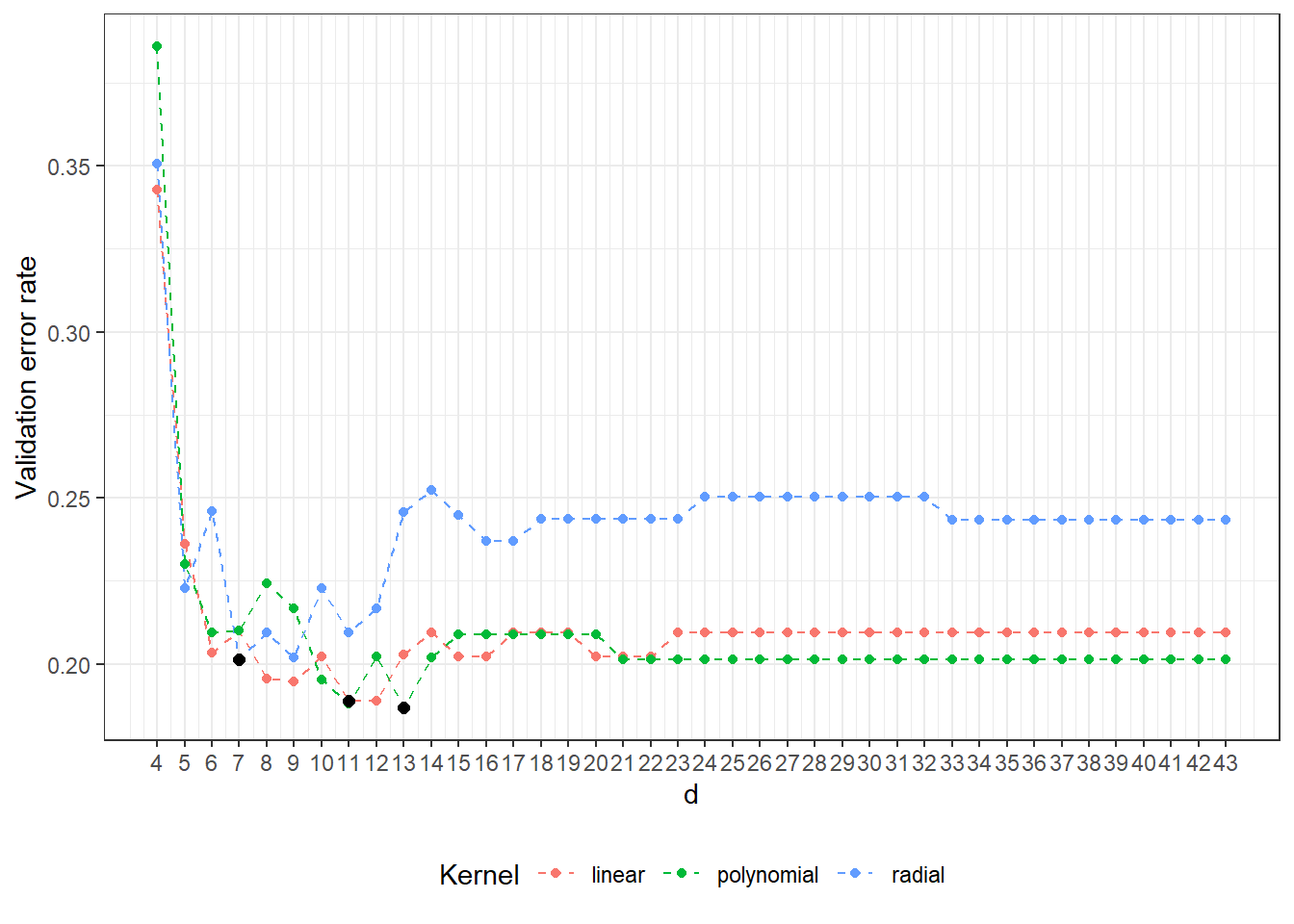
Figure 1.23: Dependency of validation error rate on the dimension of the subspace \(V_d\), separately for all three considered kernels in the SVM method. The optimal values of the dimension \(V_d\) for each kernel function are marked with black points.
Now we can train the individual classifiers on all training data and examine their performance on the test data. For each kernel function, we choose the dimension of the subspace to project onto according to the results of cross-validation.
The variable Projection stores the matrix of coefficients from the orthogonal projection, that is,
\[ \texttt{Projection} = \begin{pmatrix} \langle x_1, \Psi_1 \rangle & \langle x_2, \Psi_1 \rangle & \cdots & \langle x_n, \Psi_1 \rangle\\ \langle x_1, \Psi_2 \rangle & \langle x_2, \Psi_2 \rangle & \cdots & \langle x_n, \Psi_2 \rangle\\ \vdots & \vdots & \ddots & \vdots \\ \langle x_1, \Psi_d \rangle & \langle x_2, \Psi_d \rangle & \dots & \langle x_n, \Psi_d \rangle \end{pmatrix}_{d \times n}. \]
Code
# Prepare a data table to store results
Res <- data.frame(model = c('SVM linear - projection',
'SVM poly - projection',
'SVM rbf - projection'),
Err.train = NA,
Err.test = NA)
# Loop through each kernel
for (kernel_number in 1:3) {
kernel_type <- c('linear', 'polynomial', 'radial')[kernel_number]
# Base object
bbasis <- create.bspline.basis(rangeval = rangeval,
nbasis = d.opt[kernel_number])
# Project discrete data onto B-spline basis
Projection <- project.basis(y = rbind(
grid.data |> select(!contains('Y')),
grid.data.test |> select(!contains('Y'))) |>
as.matrix() |> t(), # Matrix of discrete data
argvals = t.seq, # Vector of arguments
basisobj = bbasis) # Basis object
# Split into training and testing data
XX.train <- t(Projection)[1:sum(split), ]
XX.test <- t(Projection)[(sum(split) + 1):length(split), ]
data.projection.train <- as.data.frame(XX.train)
data.projection.train$Y <- factor(Y.train)
data.projection.test <- as.data.frame(XX.test)
data.projection.test$Y <- factor(Y.test)
# Construct the model
clf.SVM.projection <- svm(Y ~ ., data = data.projection.train,
type = 'C-classification',
scale = TRUE,
coef0 = 1,
kernel = kernel_type)
# Accuracy on training data
predictions.train <- predict(clf.SVM.projection, newdata = data.projection.train)
presnost.train <- table(Y.train, predictions.train) |>
prop.table() |> diag() |> sum()
# Accuracy on testing data
predictions.test <- predict(clf.SVM.projection, newdata = data.projection.test)
presnost.test <- table(Y.test, predictions.test) |>
prop.table() |> diag() |> sum()
# Store results
Res[kernel_number, c(2, 3)] <- 1 - c(presnost.train, presnost.test)
}The error rate of the SVM method applied to the basis coefficients on the training data is therefore 12.14 % for the linear kernel, 12.86 % for the polynomial kernel, and 13.57 % for the Gaussian kernel. On the test data, the error rates are 20 % for the linear kernel, 25 % for the polynomial kernel, and 28.33 % for the radial kernel.
5.1.3.7.6 RKHS + SVM
In this section, we will explore another way to utilize support vector machines (SVM) for classifying functional data. Here, we will again rely on the familiar principle of first expressing functional data as finite-dimensional objects and then applying the traditional SVM method to these objects.
However, this time we will use the SVM method for the representation of functional data itself via a certain finite-dimensional object. As the name suggests, this involves a combination of two concepts: the support vector machine method and a space referred to in English literature as Reproducing Kernel Hilbert Space (RKHS). A key concept in this space is the kernel.
5.1.3.7.6.1 Implementation of the Method in R
From the last part of Theorem 1.3, we can see how to compute the representations of curves in practice. We will work with discretized data after smoothing the curves. First, let’s define a kernel for the RKHS space. We will use the Gaussian kernel with a parameter \(\gamma\). The value of this hyperparameter significantly affects the behavior and success of the method, so we must pay special attention to its choice (we select it using cross-validation).
5.1.3.7.6.2 Gaussian Kernel
Code
# Remove the last column, which contains the values of Y
data.RKHS <- grid.data[, -dim(grid.data)[2]] |> t()
# Add test data as well
data.RKHS <- cbind(data.RKHS, grid.data.test[, -dim(grid.data.test)[2]] |> t())
# Kernel and kernel matrix ... Gaussian with parameter gamma
Gauss.kernel <- function(x, y, gamma) {
return(exp(-gamma * norm(c(x - y) |> t(), type = 'F')))
}
Kernel.RKHS <- function(x, gamma) {
K <- matrix(NA, ncol = length(x), nrow = length(x))
for(i in 1:nrow(K)) {
for(j in 1:ncol(K)) {
K[i, j] <- Gauss.kernel(x = x[i], y = x[j], gamma = gamma)
}
}
return(K)
}Now let’s compute the matrix \(K_S\) along with its eigenvalues and corresponding eigenvectors.
Code
To compute the coefficients in the representation of the curves, that is, to calculate the vectors \(\hat{\boldsymbol \lambda}_l^* = \left( \hat\lambda_{1l}^*, \dots, \hat\lambda_{\hat dl}^*\right)^\top, l = 1, 2, \dots, n\), we also need the coefficients from SVM. Unlike the classification problem, we are now solving a regression problem, as we are trying to express our observed curves in some basis chosen by the kernel \(K\). Therefore, we will use the Support Vector Regression method, from which we will obtain the coefficients \(\alpha_{il}\).
Code
# Determine coefficients alpha from SVM
alpha.RKHS <- matrix(0, nrow = dim(data.RKHS)[1],
ncol = dim(data.RKHS)[2]) # Empty object
# Model
for(i in 1:dim(data.RKHS)[2]) {
df.svm <- data.frame(x = t.seq,
y = data.RKHS[, i])
svm.RKHS <- svm(y ~ x, data = df.svm,
kernel = 'radial',
type = 'eps-regression',
epsilon = 0.1,
gamma = gamma)
# Determine alpha
alpha.RKHS[svm.RKHS$index, i] <- svm.RKHS$coefs # Replace zeros with coefficients
}Now we can compute the representations of the individual curves. First, let’s choose \(\hat d\) to be the entire dimension, that is, \(\hat d = m ={}\) 101, and then determine the optimal \(\hat d\) using cross-validation.
Code
# d
d.RKHS <- dim(alpha.RKHS)[1]
# Determine the vector lambda
Lambda.RKHS <- matrix(NA,
ncol = dim(data.RKHS)[2],
nrow = d.RKHS) # Create an empty object
# Compute the representation
for(l in 1:dim(data.RKHS)[2]) {
Lambda.RKHS[, l] <- (t(eig.vectors[, 1:d.RKHS]) %*% alpha.RKHS[, l]) * eig.vals[1:d.RKHS]
}Now we have stored the vectors \(\hat{\boldsymbol \lambda}_l^*, l = 1, 2, \dots, n\) for each curve in the Lambda.RKHS matrix. We will use these vectors as representations of the given curves and classify the data based on this discretization.
Code
# Split into training and testing data
XX.train <- Lambda.RKHS[, 1:dim(grid.data)[1]]
XX.test <- Lambda.RKHS[, (dim(grid.data)[1] + 1):dim(Lambda.RKHS)[2]]
# Prepare a data frame to store results
Res <- data.frame(model = c('SVM linear - RKHS',
'SVM poly - RKHS',
'SVM rbf - RKHS'),
Err.train = NA,
Err.test = NA)
# Iterate through individual kernels
for (kernel_number in 1:3) {
kernel_type <- c('linear', 'polynomial', 'radial')[kernel_number]
data.RKHS.train <- as.data.frame(t(XX.train))
data.RKHS.train$Y <- factor(Y.train)
data.RKHS.test <- as.data.frame(t(XX.test))
data.RKHS.test$Y <- factor(Y.test)
# Construct the models
clf.SVM.RKHS <- svm(Y ~ ., data = data.RKHS.train,
type = 'C-classification',
scale = TRUE,
coef0 = 1,
kernel = kernel_type)
# Accuracy on training data
predictions.train <- predict(clf.SVM.RKHS, newdata = data.RKHS.train)
presnost.train <- table(Y.train, predictions.train) |>
prop.table() |> diag() |> sum()
# Accuracy on testing data
predictions.test <- predict(clf.SVM.RKHS, newdata = data.RKHS.test)
presnost.test <- table(Y.test, predictions.test) |>
prop.table() |> diag() |> sum()
# Store results
Res[kernel_number, c(2, 3)] <- 1 - c(presnost.train, presnost.test)
}| Model | \(\widehat{Err}_{train}\quad\quad\quad\quad\quad\) | \(\widehat{Err}_{test}\quad\quad\quad\quad\quad\) |
|---|---|---|
| SVM linear - RKHS | 0.0000 | 0.4833 |
| SVM poly - RKHS | 0.0000 | 0.4167 |
| SVM rbf - RKHS | 0.0214 | 0.3000 |
We observe that the model performs very well on the training data for all three kernels, while its success on the testing data is not good at all. It is evident that overfitting has occurred; therefore, we will use cross-validation to determine the optimal values of \(\gamma\) and \(d\).
Code
# Split training data into k parts
folds <- createMultiFolds(1:sum(split), k = k_cv, time = 1)
# Remove the last column, which contains the values of Y
data.RKHS <- grid.data[, -dim(grid.data)[2]] |> t()
# Hyperparameter values to iterate over
dimensions <- 3:40 # Reasonable range of values for d
gamma.cv <- 10^seq(-2, 3, length = 15)
# List with three components ... array for individual kernels -> linear, poly, radial
# Empty matrix where we will store individual results
# Columns will represent accuracy values for given gamma, and rows will correspond to folds
dim.names <- list(gamma = paste0('gamma:', round(gamma.cv, 3)),
d = paste0('d:', dimensions),
CV = paste0('cv:', 1:k_cv))
CV.results <- list(
SVM.l = array(NA, dim = c(length(gamma.cv), length(dimensions), k_cv),
dimnames = dim.names),
SVM.p = array(NA, dim = c(length(gamma.cv), length(dimensions), k_cv),
dimnames = dim.names),
SVM.r = array(NA, dim = c(length(gamma.cv), length(dimensions), k_cv),
dimnames = dim.names))Code
# Cross-validation
for (gamma in gamma.cv) {
K <- Kernel.RKHS(t.seq, gamma = gamma)
Eig <- eigen(K)
eig.vals <- Eig$values
eig.vectors <- Eig$vectors
alpha.RKHS <- matrix(0, nrow = dim(data.RKHS)[1], ncol = dim(data.RKHS)[2])
# Model
for(i in 1:dim(data.RKHS)[2]) {
df.svm <- data.frame(x = t.seq,
y = data.RKHS[, i])
svm.RKHS <- svm(y ~ x, data = df.svm,
kernel = 'radial',
type = 'eps-regression',
epsilon = 0.1,
gamma = gamma)
alpha.RKHS[svm.RKHS$index, i] <- svm.RKHS$coefs
}
# Iterate through dimensions
for(d.RKHS in dimensions) {
Lambda.RKHS <- matrix(NA,
ncol = dim(data.RKHS)[2],
nrow = d.RKHS)
# Calculate representation
for(l in 1:dim(data.RKHS)[2]) {
Lambda.RKHS[, l] <- (t(eig.vectors[, 1:d.RKHS]) %*%
alpha.RKHS[, l]) * eig.vals[1:d.RKHS]
}
# Iterate through folds
for (index_cv in 1:k_cv) {
# Define test and training portions for CV
fold <- folds[[index_cv]]
# Split into training and validation data
XX.train <- Lambda.RKHS[, fold]
XX.test <- Lambda.RKHS[, !(1:dim(Lambda.RKHS)[2] %in% fold)]
# Prepare a data frame to store results
Res <- data.frame(model = c('SVM linear - RKHS',
'SVM poly - RKHS',
'SVM rbf - RKHS'),
Err.test = NA)
# Iterate through individual kernels
for (kernel_number in 1:3) {
kernel_type <- c('linear', 'polynomial', 'radial')[kernel_number]
data.RKHS.train <- as.data.frame(t(XX.train))
data.RKHS.train$Y <- factor(Y.train[fold])
data.RKHS.test <- as.data.frame(t(XX.test))
data.RKHS.test$Y <- factor(Y.train[!(1:dim(Lambda.RKHS)[2] %in% fold)])
# Construct the models
clf.SVM.RKHS <- svm(Y ~ ., data = data.RKHS.train,
type = 'C-classification',
scale = TRUE,
coef0 = 1,
kernel = kernel_type)
# Accuracy on validation data
predictions.test <- predict(clf.SVM.RKHS, newdata = data.RKHS.test)
presnost.test <- table(data.RKHS.test$Y, predictions.test) |>
prop.table() |> diag() |> sum()
# Store results
Res[kernel_number, 2] <- 1 - presnost.test
}
# Store accuracies for the respective d, gamma, and fold
CV.results$SVM.l[paste0('gamma:', round(gamma, 3)),
d.RKHS - min(dimensions) + 1,
index_cv] <- Res[1, 2]
CV.results$SVM.p[paste0('gamma:', round(gamma, 3)),
d.RKHS - min(dimensions) + 1,
index_cv] <- Res[2, 2]
CV.results$SVM.r[paste0('gamma:', round(gamma, 3)),
d.RKHS - min(dimensions) + 1,
index_cv] <- Res[3, 2]
}
}
}Code
# Calculate average accuracies for each d across folds
for (n_method in 1:length(CV.results)) {
CV.results[[n_method]] <- apply(CV.results[[n_method]], c(1, 2), mean)
}
gamma.opt <- c(which.min(CV.results$SVM.l) %% length(gamma.cv),
which.min(CV.results$SVM.p) %% length(gamma.cv),
which.min(CV.results$SVM.r) %% length(gamma.cv))
gamma.opt[gamma.opt == 0] <- length(gamma.cv)
gamma.opt <- gamma.cv[gamma.opt]
d.opt <- c(which.min(t(CV.results$SVM.l)) %% length(dimensions),
which.min(t(CV.results$SVM.p)) %% length(dimensions),
which.min(t(CV.results$SVM.r)) %% length(dimensions))
d.opt[d.opt == 0] <- length(dimensions)
d.opt <- dimensions[d.opt]
err.opt.cv <- c(min(CV.results$SVM.l),
min(CV.results$SVM.p),
min(CV.results$SVM.r))
df.RKHS.res <- data.frame(d = d.opt, gamma = gamma.opt, CV = err.opt.cv,
Kernel = c('linear', 'polynomial', 'radial') |> factor(),
row.names = c('linear', 'poly', 'radial'))| \(\quad\quad\quad\quad\quad d\) | \(\quad\quad\quad\quad\quad\gamma\) | \(\widehat{Err}_{cross\_validace}\) | Model | |
|---|---|---|---|---|
| linear | 34 | 1000.0000 | 0.1271 | linear |
| poly | 37 | 1000.0000 | 0.1863 | polynomial |
| radial | 10 | 0.2683 | 0.1785 | radial |
We see that the best parameter value is \(d={}\) 34 and \(\gamma={}\) 1000 for the linear kernel with an error value calculated using 10-fold CV of 0.1271, \(d={}\) 37 and \(\gamma={}\) 1000 for the polynomial kernel with an error value calculated using 10-fold CV of 0.1863 and \(d={}\) 10 and \(\gamma={}\) 0.2683 for the radial kernel with an error value of 0.1785. For curiosity, let’s also plot the validation error function depending on the dimension \(d\) and the hyperparameter value \(\gamma\).
Code
CV.results.plot <- data.frame(d = rep(dimensions |> rep(3), each = length(gamma.cv)),
gamma = rep(gamma.cv, length(dimensions)) |> rep(3),
CV = c(c(CV.results$SVM.l),
c(CV.results$SVM.p),
c(CV.results$SVM.r)),
Kernel = rep(c('linear', 'polynomial', 'radial'),
each = length(dimensions) *
length(gamma.cv)) |> factor())
CV.results.plot |>
ggplot(aes(x = d, y = gamma, z = CV)) +
geom_contour_filled() +
scale_y_continuous(trans='log10') +
facet_wrap(~Kernel) +
theme_bw() +
labs(x = expression(d),
y = expression(gamma)) +
scale_fill_brewer(palette = "Spectral") +
geom_point(data = df.RKHS.res, aes(x = d, y = gamma),
size = 5, pch = '+')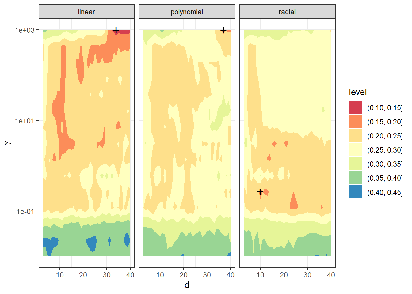
Figure 5.11: Dependency of validation error on the choice of hyperparameters \(d\) and \(\gamma\), separately for all three considered kernels in the SVM method.
Since we have already found the optimal values for the hyperparameters, we can construct the final models and determine their classification success on the test data.
Code
Code
# Prepare a data frame to store results
Res <- data.frame(model = c('SVM linear - RKHS - radial',
'SVM poly - RKHS - radial',
'SVM rbf - RKHS - radial'),
Err.train = NA,
Err.test = NA)
# Iterate through individual kernels
for (kernel_number in 1:3) {
# Calculate the K matrix
gamma <- gamma.opt[kernel_number] # Gamma value from CV
K <- Kernel.RKHS(t.seq, gamma = gamma)
# Determine eigenvalues and eigenvectors
Eig <- eigen(K)
eig.vals <- Eig$values
eig.vectors <- Eig$vectors
# Determine the alpha coefficients from SVM
alpha.RKHS <- matrix(0, nrow = dim(data.RKHS)[1],
ncol = dim(data.RKHS)[2]) # Empty object
# Model
for(i in 1:dim(data.RKHS)[2]) {
df.svm <- data.frame(x = t.seq,
y = data.RKHS[, i])
svm.RKHS <- svm(y ~ x, data = df.svm,
kernel = 'radial',
type = 'eps-regression',
epsilon = 0.1,
gamma = gamma)
# Determine alpha
alpha.RKHS[svm.RKHS$index, i] <- svm.RKHS$coefs # Replace zeros with coefficients
}
# d
d.RKHS <- d.opt[kernel_number]
# Determine the lambda vector
Lambda.RKHS <- matrix(NA,
ncol = dim(data.RKHS)[2],
nrow = d.RKHS) # Create empty object
# Compute representation
for(l in 1:dim(data.RKHS)[2]) {
Lambda.RKHS[, l] <- (t(eig.vectors[, 1:d.RKHS]) %*% alpha.RKHS[, l]) * eig.vals[1:d.RKHS]
}
# Split into training and testing data
XX.train <- Lambda.RKHS[, 1:dim(grid.data)[1]]
XX.test <- Lambda.RKHS[, (dim(grid.data)[1] + 1):dim(Lambda.RKHS)[2]]
kernel_type <- c('linear', 'polynomial', 'radial')[kernel_number]
data.RKHS.train <- as.data.frame(t(XX.train))
data.RKHS.train$Y <- factor(Y.train)
data.RKHS.test <- as.data.frame(t(XX.test))
data.RKHS.test$Y <- factor(Y.test)
# Construct models
clf.SVM.RKHS <- svm(Y ~ ., data = data.RKHS.train,
type = 'C-classification',
scale = TRUE,
coef0 = 1,
kernel = kernel_type)
# Accuracy on training data
predictions.train <- predict(clf.SVM.RKHS, newdata = data.RKHS.train)
presnost.train <- table(Y.train, predictions.train) |>
prop.table() |> diag() |> sum()
# Accuracy on testing data
predictions.test <- predict(clf.SVM.RKHS, newdata = data.RKHS.test)
presnost.test <- table(Y.test, predictions.test) |>
prop.table() |> diag() |> sum()
# Store results
Res[kernel_number, c(2, 3)] <- 1 - c(presnost.train, presnost.test)
}| Model | \(\widehat{Err}_{train}\quad\quad\quad\quad\quad\) | \(\widehat{Err}_{test}\quad\quad\quad\quad\quad\) |
|---|---|---|
| SVM linear - RKHS - radial | 0.1071 | 0.2833 |
| SVM poly - RKHS - radial | 0.1429 | 0.2667 |
| SVM rbf - RKHS - radial | 0.1357 | 0.3167 |
The error rate of the SVM method combined with the projection on the Reproducing Kernel Hilbert Space is thus equal to 10.71 % for the linear kernel, 14.29 % for the polynomial kernel, and 13.57 % for the Gaussian kernel on the training data. On the testing data, the error rate of the method is 28.33 % for the linear kernel, 26.67 % for the polynomial kernel, and 31.67 % for the radial kernel.
5.1.3.7.6.3 Polynomial Kernel
Code
# Remove the last column containing Y values
data.RKHS <- grid.data[, -dim(grid.data)[2]] |> t()
# Include test data as well
data.RKHS <- cbind(data.RKHS, grid.data.test[, -dim(grid.data.test)[2]] |> t())
# Kernel and kernel matrix ... polynomial with parameter p
Poly.kernel <- function(x, y, p) {
return((1 + x * y)^p)
}
Kernel.RKHS <- function(x, p) {
K <- matrix(NA, ncol = length(x), nrow = length(x))
for(i in 1:nrow(K)) {
for(j in 1:ncol(K)) {
K[i, j] <- Poly.kernel(x = x[i], y = x[j], p)
}
}
return(K)
}Code
# Split training data into k parts
folds <- createMultiFolds(1:sum(split), k = k_cv, time = 1)
# Remove the last column containing Y values
data.RKHS <- grid.data[, -dim(grid.data)[2]] |> t()
# Hyperparameter values to iterate over
dimensions <- 3:40 # Reasonable range of d values
poly.cv <- 2:5
# List with three components ... array for individual kernels -> linear, poly, radial
# Empty matrix to insert individual results
# Columns will hold accuracy values for given parameters
# Rows will hold values for given p and layers corresponding to folds
dim.names <- list(p = paste0('p:', poly.cv),
d = paste0('d:', dimensions),
CV = paste0('cv:', 1:k_cv))
CV.results <- list(
SVM.l = array(NA, dim = c(length(poly.cv), length(dimensions), k_cv),
dimnames = dim.names),
SVM.p = array(NA, dim = c(length(poly.cv), length(dimensions), k_cv),
dimnames = dim.names),
SVM.r = array(NA, dim = c(length(poly.cv), length(dimensions), k_cv),
dimnames = dim.names))Code
# Cross-validation
for (p in poly.cv) {
K <- Kernel.RKHS(t.seq, p = p)
Eig <- eigen(K)
eig.vals <- Eig$values
eig.vectors <- Eig$vectors
alpha.RKHS <- matrix(0, nrow = dim(data.RKHS)[1], ncol = dim(data.RKHS)[2])
# Model
for(i in 1:dim(data.RKHS)[2]) {
df.svm <- data.frame(x = t.seq,
y = data.RKHS[, i])
svm.RKHS <- svm(y ~ x, data = df.svm,
kernel = 'polynomial',
type = 'eps-regression',
epsilon = 0.1,
coef0 = 1,
degree = p)
alpha.RKHS[svm.RKHS$index, i] <- svm.RKHS$coefs
}
# Iterate through dimensions
for(d.RKHS in dimensions) {
Lambda.RKHS <- matrix(NA,
ncol = dim(data.RKHS)[2],
nrow = d.RKHS)
# Compute representation
for(l in 1:dim(data.RKHS)[2]) {
Lambda.RKHS[, l] <- (t(eig.vectors[, 1:d.RKHS]) %*%
alpha.RKHS[, l]) * eig.vals[1:d.RKHS]
}
# Iterate through folds
for (index_cv in 1:k_cv) {
# Define test and training portions for CV
fold <- folds[[index_cv]]
# Split into training and validation data
XX.train <- Lambda.RKHS[, fold]
XX.test <- Lambda.RKHS[, !(1:dim(Lambda.RKHS)[2] %in% fold)]
# Prepare a data frame to store results
Res <- data.frame(model = c('SVM linear - RKHS',
'SVM poly - RKHS',
'SVM rbf - RKHS'),
Err.test = NA)
# Iterate through individual kernels
for (kernel_number in 1:3) {
kernel_type <- c('linear', 'polynomial', 'radial')[kernel_number]
data.RKHS.train <- as.data.frame(t(XX.train))
data.RKHS.train$Y <- factor(Y.train[fold])
data.RKHS.test <- as.data.frame(t(XX.test))
data.RKHS.test$Y <- factor(Y.train[!(1:dim(Lambda.RKHS)[2] %in% fold)])
# Construct models
clf.SVM.RKHS <- svm(Y ~ ., data = data.RKHS.train,
type = 'C-classification',
scale = TRUE,
coef0 = 1,
kernel = kernel_type)
# Accuracy on validation data
predictions.test <- predict(clf.SVM.RKHS, newdata = data.RKHS.test)
presnost.test <- table(data.RKHS.test$Y, predictions.test) |>
prop.table() |> diag() |> sum()
# Store results
Res[kernel_number, 2] <- 1 - presnost.test
}
# Store accuracies in positions for given d, gamma, and fold
CV.results$SVM.l[paste0('p:', p),
d.RKHS - min(dimensions) + 1,
index_cv] <- Res[1, 2]
CV.results$SVM.p[paste0('p:', p),
d.RKHS - min(dimensions) + 1,
index_cv] <- Res[2, 2]
CV.results$SVM.r[paste0('p:', p),
d.RKHS - min(dimensions) + 1,
index_cv] <- Res[3, 2]
}
}
}Code
# Calculate average accuracies for each d across folds
for (n_method in 1:length(CV.results)) {
CV.results[[n_method]] <- apply(CV.results[[n_method]], c(1, 2), mean)
}
poly.opt <- c(which.min(CV.results$SVM.l) %% length(poly.cv),
which.min(CV.results$SVM.p) %% length(poly.cv),
which.min(CV.results$SVM.r) %% length(poly.cv))
poly.opt[poly.opt == 0] <- length(poly.cv)
poly.opt <- poly.cv[poly.opt]
d.opt <- c(which.min(t(CV.results$SVM.l)) %% length(dimensions),
which.min(t(CV.results$SVM.p)) %% length(dimensions),
which.min(t(CV.results$SVM.r)) %% length(dimensions))
d.opt[d.opt == 0] <- length(dimensions)
d.opt <- dimensions[d.opt]
err.opt.cv <- c(min(CV.results$SVM.l),
min(CV.results$SVM.p),
min(CV.results$SVM.r))
df.RKHS.res <- data.frame(d = d.opt, p = poly.opt, CV = err.opt.cv,
Kernel = c('linear', 'polynomial', 'radial') |> factor(),
row.names = c('linear', 'poly', 'radial'))| \(\quad\quad\quad\quad\quad d\) | \(\quad\quad\quad\quad\quad p\) | \(\widehat{Err}_{cross\_validation}\) | Model | |
|---|---|---|---|---|
| linear | 40 | 5 | 0.1940 | linear |
| poly | 3 | 5 | 0.1874 | polynomial |
| radial | 21 | 3 | 0.2068 | radial |
We see that the best values for parameter \(d={}\) 40 and \(p={}\) 5 are for the linear kernel with an error calculated using 10-fold CV 0.194, \(d={}\) 3 and \(p={}\) 5 for the polynomial kernel with an error calculated using 10-fold CV 0.1874, and \(d={}\) 21 and \(p={}\) 3 for the radial kernel with an error 0.2068.
Since we have found the optimal values for the hyperparameters, we can construct the final models and determine their classification success on the test data.
Code
Code
# Prepare a data frame to store results
Res <- data.frame(model = c('SVM linear - RKHS - poly',
'SVM poly - RKHS - poly',
'SVM rbf - RKHS - poly'),
Err.train = NA,
Err.test = NA)
# Iterate over the individual kernels
for (kernel_number in 1:3) {
# Calculate the matrix K
p <- poly.opt[kernel_number] # CV-derived parameter value
K <- Kernel.RKHS(t.seq, p = p)
# Determine eigenvalues and eigenvectors
Eig <- eigen(K)
eig.vals <- Eig$values
eig.vectors <- Eig$vectors
# Determine coefficients alpha from SVM
alpha.RKHS <- matrix(0, nrow = dim(data.RKHS)[1],
ncol = dim(data.RKHS)[2]) # empty object
# Model fitting
for(i in 1:dim(data.RKHS)[2]) {
df.svm <- data.frame(x = t.seq,
y = data.RKHS[, i])
svm.RKHS <- svm(y ~ x, data = df.svm,
kernel = 'polynomial',
type = 'eps-regression',
epsilon = 0.1,
coef0 = 1,
degree = p)
# Determine alpha
alpha.RKHS[svm.RKHS$index, i] <- svm.RKHS$coefs # replace zeros with coefficients
}
# d
d.RKHS <- d.opt[kernel_number]
# Determine lambda vector
Lambda.RKHS <- matrix(NA,
ncol = dim(data.RKHS)[2],
nrow = d.RKHS) # create empty object
# Calculate representation
for(l in 1:dim(data.RKHS)[2]) {
Lambda.RKHS[, l] <- (t(eig.vectors[, 1:d.RKHS]) %*% alpha.RKHS[, l]) * eig.vals[1:d.RKHS]
}
# Split into training and test data
XX.train <- Lambda.RKHS[, 1:dim(grid.data)[1]]
XX.test <- Lambda.RKHS[, (dim(grid.data)[1] + 1):dim(Lambda.RKHS)[2]]
kernel_type <- c('linear', 'polynomial', 'radial')[kernel_number]
data.RKHS.train <- as.data.frame(t(XX.train))
data.RKHS.train$Y <- factor(Y.train)
data.RKHS.test <- as.data.frame(t(XX.test))
data.RKHS.test$Y <- factor(Y.test)
# Build the models
clf.SVM.RKHS <- svm(Y ~ ., data = data.RKHS.train,
type = 'C-classification',
scale = TRUE,
coef0 = 1,
kernel = kernel_type)
# Accuracy on training data
predictions.train <- predict(clf.SVM.RKHS, newdata = data.RKHS.train)
presnost.train <- table(Y.train, predictions.train) |>
prop.table() |> diag() |> sum()
# Accuracy on test data
predictions.test <- predict(clf.SVM.RKHS, newdata = data.RKHS.test)
presnost.test <- table(Y.test, predictions.test) |>
prop.table() |> diag() |> sum()
# Store results
Res[kernel_number, c(2, 3)] <- 1 - c(presnost.train, presnost.test)
}| Model | \(\widehat{Err}_{train}\quad\quad\quad\quad\quad\) | \(\widehat{Err}_{test}\quad\quad\quad\quad\quad\) |
|---|---|---|
| SVM linear - RKHS - poly | 0.0929 | 0.3 |
| SVM poly - RKHS - poly | 0.1714 | 0.3 |
| SVM rbf - RKHS - poly | 0.1357 | 0.3 |
The error rate of the SVM method combined with projection onto the Reproducing Kernel Hilbert Space is thus on the training data equal to 9.29 % for the linear kernel, 17.14 % for the polynomial kernel, and 13.57 % for the Gaussian kernel. On the test data, the error rate of the method is 30 % for the linear kernel, 30 % for the polynomial kernel, and 30 % for the radial kernel.
5.1.3.7.6.4 Linear Kernel
Code
# Remove the last column, which contains the Y values
data.RKHS <- grid.data[, -dim(grid.data)[2]] |> t()
# Add the test data as well
data.RKHS <- cbind(data.RKHS, grid.data.test[, -dim(grid.data.test)[2]] |> t())
# Kernel and kernel matrix ... polynomial with parameter p
Linear.kernel <- function(x, y) {
return(x * y)
}
Kernel.RKHS <- function(x) {
K <- matrix(NA, ncol = length(x), nrow = length(x))
for(i in 1:nrow(K)) {
for(j in 1:ncol(K)) {
K[i, j] <- Linear.kernel(x = x[i], y = x[j])
}
}
return(K)
}Code
# Split the training data into k parts
folds <- createMultiFolds(1:sum(split), k = k_cv, time = 1)
# Remove the last column, which contains the Y values
data.RKHS <- grid.data[, -dim(grid.data)[2]] |> t()
# Values of hyperparameters that we will traverse
dimensions <- 3:40 # Reasonable range of values for d
# List with three components ... array for individual kernels -> linear, poly, radial
# Empty matrix to store the individual results
# In columns, there will be accuracy values for given d
# In rows, there will be values for layers corresponding to folds
dim.names <- list(d = paste0('d:', dimensions),
CV = paste0('cv:', 1:k_cv))
CV.results <- list(
SVM.l = array(NA, dim = c(length(dimensions), k_cv),
dimnames = dim.names),
SVM.p = array(NA, dim = c(length(dimensions), k_cv),
dimnames = dim.names),
SVM.r = array(NA, dim = c(length(dimensions), k_cv),
dimnames = dim.names))Code
# Cross-validation
K <- Kernel.RKHS(t.seq)
Eig <- eigen(K)
eig.vals <- Eig$values
eig.vectors <- Eig$vectors
alpha.RKHS <- matrix(0, nrow = dim(data.RKHS)[1], ncol = dim(data.RKHS)[2])
# Model
for(i in 1:dim(data.RKHS)[2]) {
df.svm <- data.frame(x = t.seq,
y = data.RKHS[, i])
svm.RKHS <- svm(y ~ x, data = df.svm,
kernel = 'linear',
type = 'eps-regression',
epsilon = 0.1)
alpha.RKHS[svm.RKHS$index, i] <- svm.RKHS$coefs
}
# Traverse dimensions
for(d.RKHS in dimensions) {
Lambda.RKHS <- matrix(NA,
ncol = dim(data.RKHS)[2],
nrow = d.RKHS)
# Calculation of representation
for(l in 1:dim(data.RKHS)[2]) {
Lambda.RKHS[, l] <- (t(eig.vectors[, 1:d.RKHS]) %*%
alpha.RKHS[, l]) * eig.vals[1:d.RKHS]
}
# Traverse folds
for (index_cv in 1:k_cv) {
# Define test and training portions for CV
fold <- folds[[index_cv]]
# Split into training and validation data
XX.train <- Lambda.RKHS[, fold]
XX.test <- Lambda.RKHS[, !(1:dim(Lambda.RKHS)[2] %in% fold)]
# Prepare a data table to store results
Res <- data.frame(model = c('SVM linear - RKHS',
'SVM poly - RKHS',
'SVM rbf - RKHS'),
Err.test = NA)
# Traverse individual kernels
for (kernel_number in 1:3) {
kernel_type <- c('linear', 'polynomial', 'radial')[kernel_number]
data.RKHS.train <- as.data.frame(t(XX.train))
data.RKHS.train$Y <- factor(Y.train[fold])
data.RKHS.test <- as.data.frame(t(XX.test))
data.RKHS.test$Y <- factor(Y.train[!(1:dim(Lambda.RKHS)[2] %in% fold)])
# Build models
clf.SVM.RKHS <- svm(Y ~ ., data = data.RKHS.train,
type = 'C-classification',
scale = TRUE,
coef0 = 1,
kernel = kernel_type)
# Accuracy on validation data
predictions.test <- predict(clf.SVM.RKHS, newdata = data.RKHS.test)
accuracy.test <- table(data.RKHS.test$Y, predictions.test) |>
prop.table() |> diag() |> sum()
# Store results
Res[kernel_number, 2] <- 1 - accuracy.test
}
# Store accuracies in positions for given d, gamma, and fold
CV.results$SVM.l[d.RKHS - min(dimensions) + 1,
index_cv] <- Res[1, 2]
CV.results$SVM.p[d.RKHS - min(dimensions) + 1,
index_cv] <- Res[2, 2]
CV.results$SVM.r[d.RKHS - min(dimensions) + 1,
index_cv] <- Res[3, 2]
}
}Code
# Calculate average accuracies for each d across folds
for (n_method in 1:length(CV.results)) {
CV.results[[n_method]] <- apply(CV.results[[n_method]], 1, mean)
}
d.opt <- c(which.min(t(CV.results$SVM.l)) %% length(dimensions),
which.min(t(CV.results$SVM.p)) %% length(dimensions),
which.min(t(CV.results$SVM.r)) %% length(dimensions))
d.opt[d.opt == 0] <- length(dimensions)
d.opt <- dimensions[d.opt]
err.opt.cv <- c(min(CV.results$SVM.l),
min(CV.results$SVM.p),
min(CV.results$SVM.r))
df.RKHS.res <- data.frame(d = d.opt, CV = err.opt.cv,
Kernel = c('linear', 'polynomial', 'radial') |> factor(),
row.names = c('linear', 'poly', 'radial'))| \(\quad\quad\quad\quad\quad d\) | \(\widehat{Err}_{cross\_validation}\) | Model | |
|---|---|---|---|
| linear | 9 | 0.3317 | linear |
| poly | 35 | 0.3645 | polynomial |
| radial | 10 | 0.3240 | radial |
We see that the optimal parameter value is \(d={}\) 9 for the linear kernel with an error rate calculated using 10-fold CV of 0.3317, \(d={}\) 35 for the polynomial kernel with an error rate of 0.3645, and \(d={}\) 10 for the radial kernel with an error rate of 0.324.
Now that we have found the optimal hyperparameter values, we can construct the final models and determine their classification success on the test data.
Code
Code
# Prepare a data frame to store the results
Res <- data.frame(model = c('SVM linear - RKHS - linear',
'SVM poly - RKHS - linear',
'SVM rbf - RKHS - linear'),
Err.train = NA,
Err.test = NA)
# Iterate over the individual kernels
for (kernel_number in 1:3) {
# Compute the K matrix
K <- Kernel.RKHS(t.seq)
# Determine eigenvalues and eigenvectors
Eig <- eigen(K)
eig.vals <- Eig$values
eig.vectors <- Eig$vectors
# Determine alpha coefficients from SVM
alpha.RKHS <- matrix(0, nrow = dim(data.RKHS)[1],
ncol = dim(data.RKHS)[2]) # empty object
# Model
for(i in 1:dim(data.RKHS)[2]) {
df.svm <- data.frame(x = t.seq,
y = data.RKHS[, i])
svm.RKHS <- svm(y ~ x, data = df.svm,
kernel = 'linear',
type = 'eps-regression',
epsilon = 0.1)
# Determine alpha
alpha.RKHS[svm.RKHS$index, i] <- svm.RKHS$coefs # replace zeros with coefficients
}
# d
d.RKHS <- d.opt[kernel_number]
# Determine lambda vector
Lambda.RKHS <- matrix(NA,
ncol = dim(data.RKHS)[2],
nrow = d.RKHS) # create empty object
# Calculate representation
for(l in 1:dim(data.RKHS)[2]) {
Lambda.RKHS[, l] <- (t(eig.vectors[, 1:d.RKHS]) %*% alpha.RKHS[, l]) * eig.vals[1:d.RKHS]
}
# Split into training and test data
XX.train <- Lambda.RKHS[, 1:dim(grid.data)[1]]
XX.test <- Lambda.RKHS[, (dim(grid.data)[1] + 1):dim(Lambda.RKHS)[2]]
kernel_type <- c('linear', 'polynomial', 'radial')[kernel_number]
data.RKHS.train <- as.data.frame(t(XX.train))
data.RKHS.train$Y <- factor(Y.train)
data.RKHS.test <- as.data.frame(t(XX.test))
data.RKHS.test$Y <- factor(Y.test)
# Build the model
clf.SVM.RKHS <- svm(Y ~ ., data = data.RKHS.train,
type = 'C-classification',
scale = TRUE,
coef0 = 1,
kernel = kernel_type)
# Accuracy on training data
predictions.train <- predict(clf.SVM.RKHS, newdata = data.RKHS.train)
accuracy.train <- table(Y.train, predictions.train) |>
prop.table() |> diag() |> sum()
# Accuracy on test data
predictions.test <- predict(clf.SVM.RKHS, newdata = data.RKHS.test)
accuracy.test <- table(Y.test, predictions.test) |>
prop.table() |> diag() |> sum()
# Store the results
Res[kernel_number, c(2, 3)] <- 1 - c(accuracy.train, accuracy.test)
}| Model | \(\widehat{Err}_{train}\quad\quad\quad\quad\quad\) | \(\widehat{Err}_{test}\quad\quad\quad\quad\quad\) |
|---|---|---|
| SVM linear - RKHS - linear | 0.3000 | 0.2833 |
| SVM poly - RKHS - linear | 0.3071 | 0.3000 |
| SVM rbf - RKHS - linear | 0.3071 | 0.2333 |
The error rate of the SVM method combined with projection onto the Reproducing Kernel Hilbert Space is thus 30 % for the linear kernel, 30.71 % for the polynomial kernel, and 30.71 % for the Gaussian kernel. For the test data, the error rate is 28.33 % for the linear kernel, 30 % for the polynomial kernel, and 23.33 % for the radial kernel.
5.1.3.8 Results Table
| Model | \(\widehat{Err}_{train}\quad\quad\quad\quad\quad\) | \(\widehat{Err}_{test}\quad\quad\quad\quad\quad\) |
|---|---|---|
| KNN | 0.3071 | 0.1833 |
| LDA | 0.3143 | 0.2333 |
| QDA | 0.3500 | 0.2000 |
| LR functional | 0.0500 | 0.1167 |
| LR score | 0.3143 | 0.2333 |
| Tree - discr. | 0.2643 | 0.1833 |
| Tree - score | 0.3000 | 0.2333 |
| Tree - Bbasis | 0.2643 | 0.1833 |
| RForest - discretization | 0.0000 | 0.2000 |
| RForest - score | 0.0143 | 0.3000 |
| RForest - Bbasis | 0.0000 | 0.1833 |
| SVM linear - func | 0.1571 | 0.1667 |
| SVM poly - func | 0.1214 | 0.2500 |
| SVM rbf - func | 0.1571 | 0.2333 |
| SVM linear - discretization | 0.0786 | 0.1000 |
| SVM poly - discretization | 0.1286 | 0.2333 |
| SVM rbf - discretization | 0.1429 | 0.2333 |
| SVM linear - PCA | 0.3143 | 0.2333 |
| SVM poly - PCA | 0.3143 | 0.2333 |
| SVM rbf - PCA | 0.3214 | 0.2333 |
| SVM linear - Bbasis | 0.0714 | 0.0667 |
| SVM poly - Bbasis | 0.2000 | 0.2167 |
| SVM rbf - Bbasis | 0.1286 | 0.2000 |
| SVM linear - projection | 0.1214 | 0.2000 |
| SVM poly - projection | 0.1286 | 0.2500 |
| SVM rbf - projection | 0.1357 | 0.2833 |
| SVM linear - RKHS - radial | 0.1071 | 0.2833 |
| SVM poly - RKHS - radial | 0.1429 | 0.2667 |
| SVM rbf - RKHS - radial | 0.1357 | 0.3167 |
| SVM linear - RKHS - poly | 0.0929 | 0.3000 |
| SVM poly - RKHS - poly | 0.1714 | 0.3000 |
| SVM rbf - RKHS - poly | 0.1357 | 0.3000 |
| SVM linear - RKHS - linear | 0.3000 | 0.2833 |
| SVM poly - RKHS - linear | 0.3071 | 0.3000 |
| SVM rbf - RKHS - linear | 0.3071 | 0.2333 |
5.1.4 Simulation Study
In the entire previous section, we focused only on one randomly generated set of functions from two classification classes, which we then randomly split into test and training parts. We evaluated the individual classifiers obtained using the considered methods based on test and training error rates.
Since the generated data (and their division into two parts) can differ significantly with each repetition, the error rates of the individual classification algorithms may vary greatly as well. Therefore, drawing any conclusions about the methods and comparing them based on a single generated data set can be very misleading.
For this reason, in this section, we will repeat the entire previous procedure for different generated data sets. We will store the results in a table and ultimately calculate the average characteristics of the models across individual repetitions. To ensure our conclusions are sufficiently general, we will choose the number of repetitions as \(n_{sim} = 100\).
Code
# Set seed for the pseudorandom number generator
set.seed(42)
# Number of simulations
n.sim <- 100
## List to store error rates
# Columns will represent methods
# Rows will represent individual repetitions
# The list has two entries: train and test
methods <- c('KNN', 'LDA', 'QDA', 'LR_functional', 'LR_score', 'Tree_discr',
'Tree_score', 'Tree_Bbasis', 'RF_discr', 'RF_score', 'RF_Bbasis',
'SVM linear - func', 'SVM poly - func', 'SVM rbf - func',
'SVM linear - diskr', 'SVM poly - diskr', 'SVM rbf - diskr',
'SVM linear - PCA', 'SVM poly - PCA', 'SVM rbf - PCA',
'SVM linear - Bbasis', 'SVM poly - Bbasis', 'SVM rbf - Bbasis',
'SVM linear - projection', 'SVM poly - projection',
'SVM rbf - projection', 'SVM linear - RKHS - radial',
'SVM poly - RKHS - radial', 'SVM rbf - RKHS - radial',
'SVM linear - RKHS - poly', 'SVM poly - RKHS - poly',
'SVM rbf - RKHS - poly', 'SVM linear - RKHS - linear',
'SVM poly - RKHS - linear', 'SVM rbf - RKHS - linear')
SIMULACE <- list(train = as.data.frame(matrix(NA, ncol = length(methods),
nrow = n.sim,
dimnames = list(1:n.sim, methods))),
test = as.data.frame(matrix(NA, ncol = length(methods),
nrow = n.sim,
dimnames = list(1:n.sim, methods))))
# Object to store optimal hyperparameter values determined via CV
CV_RESULTS <- data.frame(KNN_K = rep(NA, n.sim),
nharm = NA,
LR_func_n_basis = NA,
SVM_d_Linear = NA,
SVM_d_Poly = NA,
SVM_d_Radial = NA,
SVM_RKHS_radial_gamma1 = NA,
SVM_RKHS_radial_gamma2 = NA,
SVM_RKHS_radial_gamma3 = NA,
SVM_RKHS_radial_d1 = NA,
SVM_RKHS_radial_d2 = NA,
SVM_RKHS_radial_d3 = NA,
SVM_RKHS_poly_p1 = NA,
SVM_RKHS_poly_p2 = NA,
SVM_RKHS_poly_p3 = NA,
SVM_RKHS_poly_d1 = NA,
SVM_RKHS_poly_d2 = NA,
SVM_RKHS_poly_d3 = NA,
SVM_RKHS_linear_d1 = NA,
SVM_RKHS_linear_d2 = NA,
SVM_RKHS_linear_d3 = NA)Now we will repeat the entire previous section 100 times, and we will store the error rates in the list SIMULACE. We will also store the optimal hyperparameter values in the data table CV_RESULTS — for the \(K\) nearest neighbors method and for SVM, the value of dimension \(d\) in the case of projection onto the B-spline basis. Additionally, we will save all hyperparameter values for the SVM + RKHS method.
Code
# nastaveni generatoru pseudonahodnych cisel
set.seed(42)
## SIMULACE
for(sim in 1:n.sim) {
# pocet vygenerovanych pozorovani pro kazdou tridu
n <- 100
# vektor casu ekvidistantni na intervalu [0, 6]
t <- seq(0, 6, length = 51)
# pro Y = 0
X0 <- generate_values(t, funkce_0, n, 1, 2)
# pro Y = 1
X1 <- generate_values(t, funkce_1, n, 1, 2)
rangeval <- range(t)
breaks <- t
norder <- 5
bbasis <- create.bspline.basis(rangeval = rangeval,
norder = norder,
breaks = breaks)
curv.Lfd <- int2Lfd(3)
# spojeni pozorovani do jedne matice
XX <- cbind(X0, X1)
lambda.vect <- 10^seq(from = -3, to = 2, length.out = 25) # vektor lambd
gcv <- rep(NA, length = length(lambda.vect)) # prazdny vektor pro ulozebi GCV
for(index in 1:length(lambda.vect)) {
curv.Fdpar <- fdPar(bbasis, curv.Lfd, lambda.vect[index])
BSmooth <- smooth.basis(t, XX, curv.Fdpar) # vyhlazeni
gcv[index] <- mean(BSmooth$gcv) # prumer pres vsechny pozorovane krivky
}
GCV <- data.frame(
lambda = round(log10(lambda.vect), 3),
GCV = gcv
)
# najdeme hodnotu minima
lambda.opt <- lambda.vect[which.min(gcv)]
curv.fdPar <- fdPar(bbasis, curv.Lfd, lambda.opt)
BSmooth <- smooth.basis(t, XX, curv.fdPar)
XXfd <- BSmooth$fd
# vypocet derivace
XXder <- deriv.fd(XXfd, 1)
fdobjSmootheval <- eval.fd(fdobj = XXder, evalarg = t)
# rozdeleni na testovaci a trenovaci cast
split <- sample.split(XXder$fdnames$reps, SplitRatio = 0.7)
Y <- rep(c(0, 1), each = n)
X.train <- subset(XXder, split == TRUE)
X.test <- subset(XXder, split == FALSE)
Y.train <- subset(Y, split == TRUE)
Y.test <- subset(Y, split == FALSE)
x.train <- fdata(X.train)
y.train <- as.numeric(factor(Y.train))
## 1) K nejbližších sousedů
k_cv <- 10 # k-fold CV
neighbours <- 1:20 #c(1:(2 * ceiling(sqrt(length(y.train))))) # pocet sousedu
# rozdelime trenovaci data na k casti
folds <- createMultiFolds(X.train$fdnames$reps, k = k_cv, time = 1)
CV.results <- matrix(NA, nrow = length(neighbours), ncol = k_cv)
for (index in 1:k_cv) {
# definujeme danou indexovou mnozinu
fold <- folds[[index]]
x.train.cv <- subset(X.train, c(1:length(X.train$fdnames$reps)) %in% fold) |>
fdata()
y.train.cv <- subset(Y.train, c(1:length(X.train$fdnames$reps)) %in% fold) |>
factor() |> as.numeric()
x.test.cv <- subset(X.train, !c(1:length(X.train$fdnames$reps)) %in% fold) |>
fdata()
y.test.cv <- subset(Y.train, !c(1:length(X.train$fdnames$reps)) %in% fold) |>
factor() |> as.numeric()
# projdeme kazdou cast ... k-krat zopakujeme
for(neighbour in neighbours) {
# model pro konkretni volbu K
neighb.model <- classif.knn(group = y.train.cv,
fdataobj = x.train.cv,
knn = neighbour)
# predikce na validacni casti
model.neighb.predict <- predict(neighb.model,
new.fdataobj = x.test.cv)
# presnost na validacni casti
presnost <- table(y.test.cv, model.neighb.predict) |>
prop.table() |> diag() |> sum()
# presnost vlozime na pozici pro dane K a fold
CV.results[neighbour, index] <- presnost
}
}
# spocitame prumerne presnosti pro jednotliva K pres folds
CV.results <- apply(CV.results, 1, mean)
K.opt <- which.max(CV.results)
CV_RESULTS$KNN_K[sim] <- K.opt
presnost.opt.cv <- max(CV.results)
CV.results <- data.frame(K = neighbours, CV = CV.results)
neighb.model <- classif.knn(group = y.train, fdataobj = x.train, knn = K.opt)
# predikce
model.neighb.predict <- predict(neighb.model,
new.fdataobj = fdata(X.test))
presnost <- table(as.numeric(factor(Y.test)), model.neighb.predict) |>
prop.table() |>
diag() |>
sum()
RESULTS <- data.frame(model = 'KNN',
Err.train = 1 - neighb.model$max.prob,
Err.test = 1 - presnost)
## 2) Lineární diskriminační analýza
# analyza hlavnich komponent
data.PCA <- pca.fd(X.train, nharm = 10) # nharm - maximalni pocet HK
nharm <- which(cumsum(data.PCA$varprop) >= 0.9)[1] # urceni p
CV_RESULTS$nharm[sim] <- nharm
if(nharm == 1) nharm <- 2
data.PCA <- pca.fd(X.train, nharm = nharm)
data.PCA.train <- as.data.frame(data.PCA$scores) # skore prvnich p HK
data.PCA.train$Y <- factor(Y.train) # prislusnost do trid
# vypocet skoru testovacich funkci
scores <- matrix(NA, ncol = nharm, nrow = length(Y.test)) # prazdna matice
for(k in 1:dim(scores)[1]) {
xfd = X.test[k] - data.PCA$meanfd[1] # k-te pozorovani - prumerna funkce
scores[k, ] = inprod(xfd, data.PCA$harmonics)
# skalarni soucin rezidua a vlastnich funkci rho (funkcionalni hlavni komponenty)
}
data.PCA.test <- as.data.frame(scores)
data.PCA.test$Y <- factor(Y.test)
colnames(data.PCA.test) <- colnames(data.PCA.train)
# model
clf.LDA <- lda(Y ~ ., data = data.PCA.train)
# presnost na trenovacich datech
predictions.train <- predict(clf.LDA, newdata = data.PCA.train)
presnost.train <- table(data.PCA.train$Y, predictions.train$class) |>
prop.table() |> diag() |> sum()
# presnost na trenovacich datech
predictions.test <- predict(clf.LDA, newdata = data.PCA.test)
presnost.test <- table(data.PCA.test$Y, predictions.test$class) |>
prop.table() |> diag() |> sum()
Res <- data.frame(model = 'LDA',
Err.train = 1 - presnost.train,
Err.test = 1 - presnost.test)
RESULTS <- rbind(RESULTS, Res)
## 3) Kvadratická diskriminační analýza
# model
clf.QDA <- qda(Y ~ ., data = data.PCA.train)
# presnost na trenovacich datech
predictions.train <- predict(clf.QDA, newdata = data.PCA.train)
presnost.train <- table(data.PCA.train$Y, predictions.train$class) |>
prop.table() |> diag() |> sum()
# presnost na trenovacich datech
predictions.test <- predict(clf.QDA, newdata = data.PCA.test)
presnost.test <- table(data.PCA.test$Y, predictions.test$class) |>
prop.table() |> diag() |> sum()
Res <- data.frame(model = 'QDA',
Err.train = 1 - presnost.train,
Err.test = 1 - presnost.test)
RESULTS <- rbind(RESULTS, Res)
## 4) Logistická regrese
### 4.1) Funkcionální logistická regrese
# vytvorime vhodne objekty
x.train <- fdata(X.train)
y.train <- as.numeric(Y.train)
# body, ve kterych jsou funkce vyhodnoceny
tt <- x.train[["argvals"]]
dataf <- as.data.frame(y.train)
colnames(dataf) <- "Y"
# B-spline baze
basis1 <- X.train$basis
### 10-fold cross-validation
n.basis.max <- 25
n.basis <- 4:n.basis.max
k_cv <- 10 # k-fold CV
# rozdelime trenovaci data na k casti
folds <- createMultiFolds(X.train$fdnames$reps, k = k_cv, time = 1)
## prvky, ktere se behem cyklu nemeni
# body, ve kterych jsou funkce vyhodnoceny
tt <- x.train[["argvals"]]
rangeval <- range(tt)
# B-spline baze
basis1 <- X.train$basis
# vztah
f <- Y ~ x
# baze pro x
basis.x <- list("x" = basis1)
CV.results <- matrix(NA, nrow = length(n.basis), ncol = k_cv,
dimnames = list(n.basis, 1:k_cv))
for (index in 1:k_cv) {
# definujeme danou indexovou mnozinu
fold <- folds[[index]]
x.train.cv <- subset(X.train, c(1:length(X.train$fdnames$reps)) %in% fold) |>
fdata()
y.train.cv <- subset(Y.train, c(1:length(X.train$fdnames$reps)) %in% fold) |>
as.numeric()
x.test.cv <- subset(X.train, !c(1:length(X.train$fdnames$reps)) %in% fold) |>
fdata()
y.test.cv <- subset(Y.train, !c(1:length(X.train$fdnames$reps)) %in% fold) |>
as.numeric()
dataf <- as.data.frame(y.train.cv)
colnames(dataf) <- "Y"
for (i in n.basis) {
# baze pro bety
basis2 <- create.bspline.basis(rangeval = rangeval, nbasis = i)
basis.b <- list("x" = basis2)
# vstupni data do modelu
ldata <- list("df" = dataf, "x" = x.train.cv)
# binomicky model ... model logisticke regrese
model.glm <- fregre.glm(f, family = binomial(), data = ldata,
basis.x = basis.x, basis.b = basis.b)
# presnost na validacni casti
newldata = list("df" = as.data.frame(y.test.cv), "x" = x.test.cv)
predictions.valid <- predict(model.glm, newx = newldata)
predictions.valid <- data.frame(Y.pred = ifelse(predictions.valid < 1/2, 0, 1))
presnost.valid <- table(y.test.cv, predictions.valid$Y.pred) |>
prop.table() |> diag() |> sum()
# vlozime do matice
CV.results[as.character(i), as.character(index)] <- presnost.valid
}
}
# spocitame prumerne presnosti pro jednotliva n pres folds
CV.results <- apply(CV.results, 1, mean)
n.basis.opt <- n.basis[which.max(CV.results)]
CV_RESULTS$LR_func_n_basis[sim] <- n.basis.opt
presnost.opt.cv <- max(CV.results)
# optimalni model
basis2 <- create.bspline.basis(rangeval = range(tt), nbasis = n.basis.opt)
f <- Y ~ x
# baze pro x a bety
basis.x <- list("x" = basis1)
basis.b <- list("x" = basis2)
# vstupni data do modelu
dataf <- as.data.frame(y.train)
colnames(dataf) <- "Y"
ldata <- list("df" = dataf, "x" = x.train)
# binomicky model ... model logisticke regrese
model.glm <- fregre.glm(f, family = binomial(), data = ldata,
basis.x = basis.x, basis.b = basis.b)
# presnost na trenovacich datech
predictions.train <- predict(model.glm, newx = ldata)
predictions.train <- data.frame(Y.pred = ifelse(predictions.train < 1/2, 0, 1))
presnost.train <- table(Y.train, predictions.train$Y.pred) |>
prop.table() |> diag() |> sum()
# presnost na trenovacich datech
newldata = list("df" = as.data.frame(Y.test), "x" = fdata(X.test))
predictions.test <- predict(model.glm, newx = newldata)
predictions.test <- data.frame(Y.pred = ifelse(predictions.test < 1/2, 0, 1))
presnost.test <- table(Y.test, predictions.test$Y.pred) |>
prop.table() |> diag() |> sum()
Res <- data.frame(model = 'LR_functional',
Err.train = 1 - presnost.train,
Err.test = 1 - presnost.test)
RESULTS <- rbind(RESULTS, Res)
### 4.2) Logistická regrese s analýzou hlavních komponent
# model
clf.LR <- glm(Y ~ ., data = data.PCA.train, family = binomial)
# presnost na trenovacich datech
predictions.train <- predict(clf.LR, newdata = data.PCA.train, type = 'response')
predictions.train <- ifelse(predictions.train > 0.5, 1, 0)
presnost.train <- table(data.PCA.train$Y, predictions.train) |>
prop.table() |> diag() |> sum()
# presnost na trenovacich datech
predictions.test <- predict(clf.LR, newdata = data.PCA.test, type = 'response')
predictions.test <- ifelse(predictions.test > 0.5, 1, 0)
presnost.test <- table(data.PCA.test$Y, predictions.test) |>
prop.table() |> diag() |> sum()
Res <- data.frame(model = 'LR_score',
Err.train = 1 - presnost.train,
Err.test = 1 - presnost.test)
RESULTS <- rbind(RESULTS, Res)
## 5) Rozhodovací stromy
### 5.1) Diskretizace intervalu
# posloupnost bodu, ve kterych funkce vyhodnotime
t.seq <- seq(0, 6, length = 101)
grid.data <- eval.fd(fdobj = X.train, evalarg = t.seq)
grid.data <- as.data.frame(t(grid.data)) # transpozice kvuli funkcim v radku
grid.data$Y <- Y.train |> factor()
grid.data.test <- eval.fd(fdobj = X.test, evalarg = t.seq)
grid.data.test <- as.data.frame(t(grid.data.test))
grid.data.test$Y <- Y.test |> factor()
# sestrojeni modelu
clf.tree <- train(Y ~ ., data = grid.data,
method = "rpart",
trControl = trainControl(method = "CV", number = 10),
metric = "Accuracy")
# presnost na trenovacich datech
predictions.train <- predict(clf.tree, newdata = grid.data)
presnost.train <- table(Y.train, predictions.train) |>
prop.table() |> diag() |> sum()
# presnost na trenovacich datech
predictions.test <- predict(clf.tree, newdata = grid.data.test)
presnost.test <- table(Y.test, predictions.test) |>
prop.table() |> diag() |> sum()
Res <- data.frame(model = 'Tree_discr',
Err.train = 1 - presnost.train,
Err.test = 1 - presnost.test)
RESULTS <- rbind(RESULTS, Res)
### 5.2) Skóre hlavních komponent
# sestrojeni modelu
clf.tree.PCA <- train(Y ~ ., data = data.PCA.train,
method = "rpart",
trControl = trainControl(method = "CV", number = 10),
metric = "Accuracy")
# presnost na trenovacich datech
predictions.train <- predict(clf.tree.PCA, newdata = data.PCA.train)
presnost.train <- table(Y.train, predictions.train) |>
prop.table() |> diag() |> sum()
# presnost na trenovacich datech
predictions.test <- predict(clf.tree.PCA, newdata = data.PCA.test)
presnost.test <- table(Y.test, predictions.test) |>
prop.table() |> diag() |> sum()
Res <- data.frame(model = 'Tree_score',
Err.train = 1 - presnost.train,
Err.test = 1 - presnost.test)
RESULTS <- rbind(RESULTS, Res)
### 5.3) Bázové koeficienty
# trenovaci dataset
data.Bbasis.train <- t(X.train$coefs) |> as.data.frame()
data.Bbasis.train$Y <- factor(Y.train)
# testovaci dataset
data.Bbasis.test <- t(X.test$coefs) |> as.data.frame()
data.Bbasis.test$Y <- factor(Y.test)
# sestrojeni modelu
clf.tree.Bbasis <- train(Y ~ ., data = data.Bbasis.train,
method = "rpart",
trControl = trainControl(method = "CV", number = 10),
metric = "Accuracy")
# presnost na trenovacich datech
predictions.train <- predict(clf.tree.Bbasis, newdata = data.Bbasis.train)
presnost.train <- table(Y.train, predictions.train) |>
prop.table() |> diag() |> sum()
# presnost na trenovacich datech
predictions.test <- predict(clf.tree.Bbasis, newdata = data.Bbasis.test)
presnost.test <- table(Y.test, predictions.test) |>
prop.table() |> diag() |> sum()
Res <- data.frame(model = 'Tree_Bbasis',
Err.train = 1 - presnost.train,
Err.test = 1 - presnost.test)
RESULTS <- rbind(RESULTS, Res)
## 6) Náhodné lesy
### 6.1) Diskretizace intervalu
# sestrojeni modelu
clf.RF <- randomForest(Y ~ ., data = grid.data,
ntree = 500, # pocet stromu
importance = TRUE,
nodesize = 5)
# presnost na trenovacich datech
predictions.train <- predict(clf.RF, newdata = grid.data)
presnost.train <- table(Y.train, predictions.train) |>
prop.table() |> diag() |> sum()
# presnost na trenovacich datech
predictions.test <- predict(clf.RF, newdata = grid.data.test)
presnost.test <- table(Y.test, predictions.test) |>
prop.table() |> diag() |> sum()
Res <- data.frame(model = 'RF_discr',
Err.train = 1 - presnost.train,
Err.test = 1 - presnost.test)
RESULTS <- rbind(RESULTS, Res)
### 6.2) Skóre hlavních komponent
# sestrojeni modelu
clf.RF.PCA <- randomForest(Y ~ ., data = data.PCA.train,
ntree = 500, # pocet stromu
importance = TRUE,
nodesize = 5)
# presnost na trenovacich datech
predictions.train <- predict(clf.RF.PCA, newdata = data.PCA.train)
presnost.train <- table(Y.train, predictions.train) |>
prop.table() |> diag() |> sum()
# presnost na trenovacich datech
predictions.test <- predict(clf.RF.PCA, newdata = data.PCA.test)
presnost.test <- table(Y.test, predictions.test) |>
prop.table() |> diag() |> sum()
Res <- data.frame(model = 'RF_score',
Err.train = 1 - presnost.train,
Err.test = 1 - presnost.test)
RESULTS <- rbind(RESULTS, Res)
### 6.3) Bázové koeficienty
# sestrojeni modelu
clf.RF.Bbasis <- randomForest(Y ~ ., data = data.Bbasis.train,
ntree = 500, # pocet stromu
importance = TRUE,
nodesize = 5)
# presnost na trenovacich datech
predictions.train <- predict(clf.RF.Bbasis, newdata = data.Bbasis.train)
presnost.train <- table(Y.train, predictions.train) |>
prop.table() |> diag() |> sum()
# presnost na trenovacich datech
predictions.test <- predict(clf.RF.Bbasis, newdata = data.Bbasis.test)
presnost.test <- table(Y.test, predictions.test) |>
prop.table() |> diag() |> sum()
Res <- data.frame(model = 'RF_Bbasis',
Err.train = 1 - presnost.train,
Err.test = 1 - presnost.test)
RESULTS <- rbind(RESULTS, Res)
## 7) SVM
# normovani dat
norms <- c()
for (i in 1:dim(XXder$coefs)[2]) {
norms <- c(norms, as.numeric(1 / norm.fd(XXder[i])))
}
XXfd_norm <- XXder
XXfd_norm$coefs <- XXfd_norm$coefs * matrix(norms,
ncol = dim(XXder$coefs)[2],
nrow = dim(XXder$coefs)[1],
byrow = T)
# rozdeleni na testovaci a trenovaci cast
X.train_norm <- subset(XXfd_norm, split == TRUE)
X.test_norm <- subset(XXfd_norm, split == FALSE)
Y.train_norm <- subset(Y, split == TRUE)
Y.test_norm <- subset(Y, split == FALSE)
grid.data <- eval.fd(fdobj = X.train_norm, evalarg = t.seq)
grid.data <- as.data.frame(t(grid.data))
grid.data$Y <- Y.train_norm |> factor()
grid.data.test <- eval.fd(fdobj = X.test_norm, evalarg = t.seq)
grid.data.test <- as.data.frame(t(grid.data.test))
grid.data.test$Y <- Y.test_norm |> factor()
### 7.0) SVM for functional data
# vytvorime vhodne objekty
x.train <- fdata(X.train_norm)
y.train <- as.factor(Y.train_norm)
# body, ve kterych jsou funkce vyhodnoceny
tt <- x.train[["argvals"]]
dataf <- as.data.frame(y.train)
colnames(dataf) <- "Y"
# B-spline baze
basis1 <- X.train_norm$basis
# formula
f <- Y ~ x
# baze pro x
basis.x <- list("x" = basis1)
# vstupni data do modelu
ldata <- list("df" = dataf, "x" = x.train)
model.svm.f_l <- classif.svm(formula = f,
data = ldata,
basis.x = basis.x,
kernel = 'linear',
type = 'C-classification',
scale = TRUE,
cost = 10)
model.svm.f_p <- classif.svm(formula = f,
data = ldata,
basis.x = basis.x,
kernel = 'polynomial',
type = 'C-classification',
scale = TRUE,
degree = 3,
coef0 = 1,
cost = 10)
model.svm.f_r <- classif.svm(formula = f,
data = ldata,
basis.x = basis.x,
kernel = 'radial',
type = 'C-classification',
scale = TRUE,
gamma = 0.001,
cost = 100)
# presnost na trenovacich datech
newdat <- list("x" = x.train)
predictions.train.l <- predict(model.svm.f_l, newdat, type = 'class')
presnost.train.l <- mean(factor(Y.train_norm) == predictions.train.l)
predictions.train.p <- predict(model.svm.f_p, newdat, type = 'class')
presnost.train.p <- mean(factor(Y.train_norm) == predictions.train.p)
predictions.train.r <- predict(model.svm.f_r, newdat, type = 'class')
presnost.train.r <- mean(factor(Y.train_norm) == predictions.train.r)
# presnost na testovacich datech
newdat <- list("x" = fdata(X.test_norm))
predictions.test.l <- predict(model.svm.f_l, newdat, type = 'class')
presnost.test.l <- mean(factor(Y.test_norm) == predictions.test.l)
predictions.test.p <- predict(model.svm.f_p, newdat, type = 'class')
presnost.test.p <- mean(factor(Y.test_norm) == predictions.test.p)
predictions.test.r <- predict(model.svm.f_r, newdat, type = 'class')
presnost.test.r <- mean(factor(Y.test_norm) == predictions.test.r)
Res <- data.frame(model = c('SVM linear - func',
'SVM poly - func',
'SVM rbf - func'),
Err.train = 1 - c(presnost.train.l, presnost.train.p, presnost.train.r),
Err.test = 1 - c(presnost.test.l, presnost.test.p, presnost.test.r))
RESULTS <- rbind(RESULTS, Res)
### 7.1) Diskretizace intervalu
clf.SVM.l <- svm(Y ~ ., data = grid.data,
type = 'C-classification',
scale = TRUE,
cost = 25,
kernel = 'linear')
clf.SVM.p <- svm(Y ~ ., data = grid.data,
type = 'C-classification',
scale = TRUE,
coef0 = 1,
cost = 0.7,
kernel = 'polynomial')
clf.SVM.r <- svm(Y ~ ., data = grid.data,
type = 'C-classification',
scale = TRUE,
cost = 55,
gamma = 0.0005,
kernel = 'radial')
# presnost na trenovacich datech
predictions.train.l <- predict(clf.SVM.l, newdata = grid.data)
presnost.train.l <- table(Y.train, predictions.train.l) |>
prop.table() |> diag() |> sum()
predictions.train.p <- predict(clf.SVM.p, newdata = grid.data)
presnost.train.p <- table(Y.train, predictions.train.p) |>
prop.table() |> diag() |> sum()
predictions.train.r <- predict(clf.SVM.r, newdata = grid.data)
presnost.train.r <- table(Y.train, predictions.train.r) |>
prop.table() |> diag() |> sum()
# presnost na testovacich datech
predictions.test.l <- predict(clf.SVM.l, newdata = grid.data.test)
presnost.test.l <- table(Y.test, predictions.test.l) |>
prop.table() |> diag() |> sum()
predictions.test.p <- predict(clf.SVM.p, newdata = grid.data.test)
presnost.test.p <- table(Y.test, predictions.test.p) |>
prop.table() |> diag() |> sum()
predictions.test.r <- predict(clf.SVM.r, newdata = grid.data.test)
presnost.test.r <- table(Y.test, predictions.test.r) |>
prop.table() |> diag() |> sum()
Res <- data.frame(model = c('SVM linear - diskr',
'SVM poly - diskr',
'SVM rbf - diskr'),
Err.train = 1 - c(presnost.train.l,
presnost.train.p, presnost.train.r),
Err.test = 1 - c(presnost.test.l,
presnost.test.p, presnost.test.r))
RESULTS <- rbind(RESULTS, Res)
### 7.2) Skóre hlavních komponent
# sestrojeni modelu
clf.SVM.l.PCA <- svm(Y ~ ., data = data.PCA.train,
type = 'C-classification',
scale = TRUE,
cost = 0.1,
kernel = 'linear')
clf.SVM.p.PCA <- svm(Y ~ ., data = data.PCA.train,
type = 'C-classification',
scale = TRUE,
coef0 = 1,
cost = 0.01,
kernel = 'polynomial')
clf.SVM.r.PCA <- svm(Y ~ ., data = data.PCA.train,
type = 'C-classification',
scale = TRUE,
cost = 1,
gamma = 0.01,
kernel = 'radial')
# presnost na trenovacich datech
predictions.train.l <- predict(clf.SVM.l.PCA, newdata = data.PCA.train)
presnost.train.l <- table(data.PCA.train$Y, predictions.train.l) |>
prop.table() |> diag() |> sum()
predictions.train.p <- predict(clf.SVM.p.PCA, newdata = data.PCA.train)
presnost.train.p <- table(data.PCA.train$Y, predictions.train.p) |>
prop.table() |> diag() |> sum()
predictions.train.r <- predict(clf.SVM.r.PCA, newdata = data.PCA.train)
presnost.train.r <- table(data.PCA.train$Y, predictions.train.r) |>
prop.table() |> diag() |> sum()
# presnost na testovacich datech
predictions.test.l <- predict(clf.SVM.l.PCA, newdata = data.PCA.test)
presnost.test.l <- table(data.PCA.test$Y, predictions.test.l) |>
prop.table() |> diag() |> sum()
predictions.test.p <- predict(clf.SVM.p.PCA, newdata = data.PCA.test)
presnost.test.p <- table(data.PCA.test$Y, predictions.test.p) |>
prop.table() |> diag() |> sum()
predictions.test.r <- predict(clf.SVM.r.PCA, newdata = data.PCA.test)
presnost.test.r <- table(data.PCA.test$Y, predictions.test.r) |>
prop.table() |> diag() |> sum()
Res <- data.frame(model = c('SVM linear - PCA',
'SVM poly - PCA',
'SVM rbf - PCA'),
Err.train = 1 - c(presnost.train.l,
presnost.train.p, presnost.train.r),
Err.test = 1 - c(presnost.test.l,
presnost.test.p, presnost.test.r))
RESULTS <- rbind(RESULTS, Res)
### 7.3) Bázové koeficienty
# sestrojeni modelu
clf.SVM.l.Bbasis <- svm(Y ~ ., data = data.Bbasis.train,
type = 'C-classification',
scale = TRUE,
cost = 50,
kernel = 'linear')
clf.SVM.p.Bbasis <- svm(Y ~ ., data = data.Bbasis.train,
type = 'C-classification',
scale = TRUE,
coef0 = 1,
cost = 0.1,
kernel = 'polynomial')
clf.SVM.r.Bbasis <- svm(Y ~ ., data = data.Bbasis.train,
type = 'C-classification',
scale = TRUE,
cost = 100,
gamma = 0.001,
kernel = 'radial')
# presnost na trenovacich datech
predictions.train.l <- predict(clf.SVM.l.Bbasis, newdata = data.Bbasis.train)
presnost.train.l <- table(Y.train, predictions.train.l) |>
prop.table() |> diag() |> sum()
predictions.train.p <- predict(clf.SVM.p.Bbasis, newdata = data.Bbasis.train)
presnost.train.p <- table(Y.train, predictions.train.p) |>
prop.table() |> diag() |> sum()
predictions.train.r <- predict(clf.SVM.r.Bbasis, newdata = data.Bbasis.train)
presnost.train.r <- table(Y.train, predictions.train.r) |>
prop.table() |> diag() |> sum()
# presnost na trenovacich datech
predictions.test.l <- predict(clf.SVM.l.Bbasis, newdata = data.Bbasis.test)
presnost.test.l <- table(Y.test, predictions.test.l) |>
prop.table() |> diag() |> sum()
predictions.test.p <- predict(clf.SVM.p.Bbasis, newdata = data.Bbasis.test)
presnost.test.p <- table(Y.test, predictions.test.p) |>
prop.table() |> diag() |> sum()
predictions.test.r <- predict(clf.SVM.r.Bbasis, newdata = data.Bbasis.test)
presnost.test.r <- table(Y.test, predictions.test.r) |>
prop.table() |> diag() |> sum()
Res <- data.frame(model = c('SVM linear - Bbasis',
'SVM poly - Bbasis',
'SVM rbf - Bbasis'),
Err.train = 1 - c(presnost.train.l,
presnost.train.p, presnost.train.r),
Err.test = 1 - c(presnost.test.l,
presnost.test.p, presnost.test.r))
RESULTS <- rbind(RESULTS, Res)
### 7.4) Projekce na B-splinovou bázi
# hodnoty pro B-splinovou bazi
rangeval <- range(t)
norder <- 4
n_basis_min <- norder
n_basis_max <- 20 #length(t) + norder - 2 - 10
dimensions <- n_basis_min:n_basis_max
folds <- createMultiFolds(1:sum(split), k = k_cv, time = 1)
CV.results <- list(SVM.l = matrix(NA, nrow = length(dimensions), ncol = k_cv),
SVM.p = matrix(NA, nrow = length(dimensions), ncol = k_cv),
SVM.r = matrix(NA, nrow = length(dimensions), ncol = k_cv))
for (d in dimensions) {
bbasis <- create.bspline.basis(rangeval = rangeval,
nbasis = d)
Projection <- project.basis(y = grid.data |> select(!contains('Y')) |>
as.matrix() |> t(),
argvals = t.seq, basisobj = bbasis)
# rozdeleni na trenovaci a testovaci data v ramci CV
XX.train <- t(Projection)
for (index_cv in 1:k_cv) {
fold <- folds[[index_cv]]
cv_sample <- 1:dim(XX.train)[1] %in% fold
data.projection.train.cv <- as.data.frame(XX.train[cv_sample, ])
data.projection.train.cv$Y <- factor(Y.train[cv_sample])
data.projection.test.cv <- as.data.frame(XX.train[!cv_sample, ])
Y.test.cv <- Y.train[!cv_sample]
data.projection.test.cv$Y <- factor(Y.test.cv)
# sestrojeni modelu
clf.SVM.l.projection <- svm(Y ~ ., data = data.projection.train.cv,
type = 'C-classification',
scale = TRUE,
kernel = 'linear')
clf.SVM.p.projection <- svm(Y ~ ., data = data.projection.train.cv,
type = 'C-classification',
scale = TRUE,
coef0 = 1,
kernel = 'polynomial')
clf.SVM.r.projection <- svm(Y ~ ., data = data.projection.train.cv,
type = 'C-classification',
scale = TRUE,
kernel = 'radial')
# presnost na validacnich datech
## linear kernel
predictions.test.l <- predict(clf.SVM.l.projection,
newdata = data.projection.test.cv)
presnost.test.l <- table(Y.test.cv, predictions.test.l) |>
prop.table() |> diag() |> sum()
## polynomial kernel
predictions.test.p <- predict(clf.SVM.p.projection,
newdata = data.projection.test.cv)
presnost.test.p <- table(Y.test.cv, predictions.test.p) |>
prop.table() |> diag() |> sum()
## radial kernel
predictions.test.r <- predict(clf.SVM.r.projection,
newdata = data.projection.test.cv)
presnost.test.r <- table(Y.test.cv, predictions.test.r) |>
prop.table() |> diag() |> sum()
# presnosti vlozime na pozice pro dane d a fold
CV.results$SVM.l[d - min(dimensions) + 1, index_cv] <- presnost.test.l
CV.results$SVM.p[d - min(dimensions) + 1, index_cv] <- presnost.test.p
CV.results$SVM.r[d - min(dimensions) + 1, index_cv] <- presnost.test.r
}
}
# spocitame prumerne presnosti pro jednotliva d pres folds
for (n_method in 1:length(CV.results)) {
CV.results[[n_method]] <- apply(CV.results[[n_method]], 1, mean)
}
d.opt <- c(which.max(CV.results$SVM.l) + n_basis_min - 1,
which.max(CV.results$SVM.p) + n_basis_min - 1,
which.max(CV.results$SVM.r) + n_basis_min - 1)
# ulozime optimalni d do datove tabulky
CV_RESULTS[sim, 4:6] <- d.opt
# pripravime si datovou tabulku pro ulozeni vysledku
Res <- data.frame(model = c('SVM linear - projection',
'SVM poly - projection',
'SVM rbf - projection'),
Err.train = NA,
Err.test = NA)
for (kernel_number in 1:3) {
kernel_type <- c('linear', 'polynomial', 'radial')[kernel_number]
bbasis <- create.bspline.basis(rangeval = rangeval,
nbasis = d.opt[kernel_number])
Projection <- project.basis(y = rbind(
grid.data |> select(!contains('Y')),
grid.data.test |> select(!contains('Y'))) |>
as.matrix() |> t(), argvals = t.seq, basisobj = bbasis)
XX.train <- t(Projection)[1:sum(split), ]
XX.test <- t(Projection)[(sum(split) + 1):length(split), ]
data.projection.train <- as.data.frame(XX.train)
data.projection.train$Y <- factor(Y.train)
data.projection.test <- as.data.frame(XX.test)
data.projection.test$Y <- factor(Y.test)
# sestrojeni modelu
clf.SVM.projection <- svm(Y ~ ., data = data.projection.train,
type = 'C-classification',
scale = TRUE,
coef0 = 1,
kernel = kernel_type)
# presnost na trenovacich datech
predictions.train <- predict(clf.SVM.projection, newdata = data.projection.train)
presnost.train <- table(Y.train, predictions.train) |>
prop.table() |> diag() |> sum()
# presnost na trenovacich datech
predictions.test <- predict(clf.SVM.projection, newdata = data.projection.test)
presnost.test <- table(Y.test, predictions.test) |>
prop.table() |> diag() |> sum()
# ulozeni vysledku
Res[kernel_number, c(2, 3)] <- 1 - c(presnost.train, presnost.test)
}
RESULTS <- rbind(RESULTS, Res)
## 7.5) SVM + RKHS
### Gaussovo jadro
# jadro a jadrova matice ... Gaussovske s parametrem gamma
Gauss.kernel <- function(x, y, gamma) {
return(exp(-gamma * norm(c(x - y) |> t(), type = 'F')))
}
Kernel.RKHS <- function(x, gamma) {
K <- matrix(NA, ncol = length(x), nrow = length(x))
for(i in 1:nrow(K)) {
for(j in 1:ncol(K)) {
K[i, j] <- Gauss.kernel(x = x[i], y = x[j], gamma = gamma)
}
}
return(K)
}
# rozdelime trenovaci data na k casti
folds <- createMultiFolds(1:sum(split), k = k_cv, time = 1)
# odstranime posledni sloupec, ve kterem jsou hodnoty Y
data.RKHS <- grid.data[, -dim(grid.data)[2]] |> t()
# hodnoty hyperparametru, ktere budeme prochazet
dimensions <- seq(5, 40, by = 5) # rozumny rozsah hodnot d
gamma.cv <- 10^seq(-1, 2, length = 5)
# list se tremi slozkami ... array pro jednotlive jadra -> linear, poly, radial
# prazdna matice, do ktere vlozime jednotlive vysledky
# ve sloupcich budou hodnoty presnosti pro dane
# v radcich budou hodnoty pro danou gamma a vrstvy odpovidaji folds
dim.names <- list(gamma = paste0('gamma:', round(gamma.cv, 3)),
d = paste0('d:', dimensions),
CV = paste0('cv:', 1:k_cv))
CV.results <- list(
SVM.l = array(NA, dim = c(length(gamma.cv), length(dimensions), k_cv),
dimnames = dim.names),
SVM.p = array(NA, dim = c(length(gamma.cv), length(dimensions), k_cv),
dimnames = dim.names),
SVM.r = array(NA, dim = c(length(gamma.cv), length(dimensions), k_cv),
dimnames = dim.names))
# samotna CV
for (gamma in gamma.cv) {
K <- Kernel.RKHS(t.seq, gamma = gamma)
Eig <- eigen(K)
eig.vals <- Eig$values
eig.vectors <- Eig$vectors
alpha.RKHS <- matrix(0, nrow = dim(data.RKHS)[1], ncol = dim(data.RKHS)[2])
# model
for(i in 1:dim(data.RKHS)[2]) {
df.svm <- data.frame(x = t.seq,
y = data.RKHS[, i])
svm.RKHS <- svm(y ~ x, data = df.svm,
kernel = 'radial',
type = 'eps-regression',
epsilon = 0.1,
gamma = gamma)
alpha.RKHS[svm.RKHS$index, i] <- svm.RKHS$coefs
}
# projdeme dimenze
for(d.RKHS in dimensions) {
Lambda.RKHS <- matrix(NA,
ncol = dim(data.RKHS)[2],
nrow = d.RKHS)
# vypocet reprezentace
for(l in 1:dim(data.RKHS)[2]) {
Lambda.RKHS[, l] <- (t(eig.vectors[, 1:d.RKHS]) %*%
alpha.RKHS[, l]) * eig.vals[1:d.RKHS]
}
# projdeme folds
for (index_cv in 1:k_cv) {
# definice testovaci a trenovaci casti pro CV
fold <- folds[[index_cv]]
# rozdeleni na trenovaci a validacni data
XX.train <- Lambda.RKHS[, fold]
XX.test <- Lambda.RKHS[, !(1:dim(Lambda.RKHS)[2] %in% fold)]
# pripravime si datovou tabulku pro ulozeni vysledku
Res <- data.frame(model = c('SVM linear - RKHS',
'SVM poly - RKHS',
'SVM rbf - RKHS'),
Err.test = NA)
# projdeme jednotliva jadra
for (kernel_number in 1:3) {
kernel_type <- c('linear', 'polynomial', 'radial')[kernel_number]
data.RKHS.train <- as.data.frame(t(XX.train))
data.RKHS.train$Y <- factor(Y.train[fold])
data.RKHS.test <- as.data.frame(t(XX.test))
data.RKHS.test$Y <- factor(Y.train[!(1:dim(Lambda.RKHS)[2] %in% fold)])
# sestrojeni modelu
clf.SVM.RKHS <- svm(Y ~ ., data = data.RKHS.train,
type = 'C-classification',
scale = TRUE,
coef0 = 1,
kernel = kernel_type)
# presnost na validacnich datech
predictions.test <- predict(clf.SVM.RKHS, newdata = data.RKHS.test)
presnost.test <- table(data.RKHS.test$Y, predictions.test) |>
prop.table() |> diag() |> sum()
# ulozeni vysledku
Res[kernel_number, 2] <- 1 - presnost.test
}
# presnosti vlozime na pozice pro dane d, gamma a fold
CV.results$SVM.l[paste0('gamma:', round(gamma, 3)),
paste0('d:', d.RKHS),
index_cv] <- Res[1, 2]
CV.results$SVM.p[paste0('gamma:', round(gamma, 3)),
paste0('d:', d.RKHS),
index_cv] <- Res[2, 2]
CV.results$SVM.r[paste0('gamma:', round(gamma, 3)),
paste0('d:', d.RKHS),
index_cv] <- Res[3, 2]
}
}
}
# spocitame prumerne presnosti pro jednotliva d pres folds
for (n_method in 1:length(CV.results)) {
CV.results[[n_method]] <- apply(CV.results[[n_method]], c(1, 2), mean)
}
gamma.opt <- c(which.min(CV.results$SVM.l) %% length(gamma.cv),
which.min(CV.results$SVM.p) %% length(gamma.cv),
which.min(CV.results$SVM.r) %% length(gamma.cv))
gamma.opt[gamma.opt == 0] <- length(gamma.cv)
gamma.opt <- gamma.cv[gamma.opt]
d.opt <- c(which.min(t(CV.results$SVM.l)) %% length(dimensions),
which.min(t(CV.results$SVM.p)) %% length(dimensions),
which.min(t(CV.results$SVM.r)) %% length(dimensions))
d.opt[d.opt == 0] <- length(dimensions)
d.opt <- dimensions[d.opt]
err.opt.cv <- c(min(CV.results$SVM.l),
min(CV.results$SVM.p),
min(CV.results$SVM.r))
df.RKHS.res <- data.frame(d = d.opt, gamma = gamma.opt, CV = err.opt.cv,
Kernel = c('linear', 'polynomial', 'radial') |> factor(),
row.names = c('linear', 'poly', 'radial'))
CV_RESULTS[sim, 7:9] <- gamma.opt
CV_RESULTS[sim, 10:12] <- d.opt
# odstranime posledni sloupec, ve kterem jsou hodnoty Y
data.RKHS <- grid.data[, -dim(grid.data)[2]] |> t()
# pridame i testovaci data
data.RKHS <- cbind(data.RKHS, grid.data.test[, -dim(grid.data.test)[2]] |> t())
# pripravime si datovou tabulku pro ulozeni vysledku
Res <- data.frame(model = c('SVM linear - RKHS - radial',
'SVM poly - RKHS - radial',
'SVM rbf - RKHS - radial'),
Err.train = NA,
Err.test = NA)
# projdeme jednotliva jadra
for (kernel_number in 1:3) {
# spocitame matici K
gamma <- gamma.opt[kernel_number] # hodnota gamma pomoci CV
K <- Kernel.RKHS(t.seq, gamma = gamma)
# urcime vlastni cisla a vektory
Eig <- eigen(K)
eig.vals <- Eig$values
eig.vectors <- Eig$vectors
# urceni koeficientu alpha z SVM
alpha.RKHS <- matrix(0, nrow = dim(data.RKHS)[1],
ncol = dim(data.RKHS)[2]) # prazdny objekt
# model
for(i in 1:dim(data.RKHS)[2]) {
df.svm <- data.frame(x = t.seq,
y = data.RKHS[, i])
svm.RKHS <- svm(y ~ x, data = df.svm,
kernel = 'radial',
type = 'eps-regression',
epsilon = 0.1,
gamma = gamma)
# urceni alpha
alpha.RKHS[svm.RKHS$index, i] <- svm.RKHS$coefs # nahrazeni nul koeficienty
}
# d
d.RKHS <- d.opt[kernel_number]
# urceni vektoru lambda
Lambda.RKHS <- matrix(NA,
ncol = dim(data.RKHS)[2],
nrow = d.RKHS) # vytvoreni prazdneho objektu
# vypocet reprezentace
for(l in 1:dim(data.RKHS)[2]) {
Lambda.RKHS[, l] <- (t(eig.vectors[, 1:d.RKHS]) %*% alpha.RKHS[, l]) * eig.vals[1:d.RKHS]
}
# rozdeleni na trenovaci a testovaci data
XX.train <- Lambda.RKHS[, 1:dim(grid.data)[1]]
XX.test <- Lambda.RKHS[, (dim(grid.data)[1] + 1):dim(Lambda.RKHS)[2]]
kernel_type <- c('linear', 'polynomial', 'radial')[kernel_number]
data.RKHS.train <- as.data.frame(t(XX.train))
data.RKHS.train$Y <- factor(Y.train)
data.RKHS.test <- as.data.frame(t(XX.test))
data.RKHS.test$Y <- factor(Y.test)
# sestrojeni modelu
clf.SVM.RKHS <- svm(Y ~ ., data = data.RKHS.train,
type = 'C-classification',
scale = TRUE,
coef0 = 1,
kernel = kernel_type)
# presnost na trenovacich datech
predictions.train <- predict(clf.SVM.RKHS, newdata = data.RKHS.train)
presnost.train <- table(Y.train, predictions.train) |>
prop.table() |> diag() |> sum()
# presnost na testovacich datech
predictions.test <- predict(clf.SVM.RKHS, newdata = data.RKHS.test)
presnost.test <- table(Y.test, predictions.test) |>
prop.table() |> diag() |> sum()
# ulozeni vysledku
Res[kernel_number, c(2, 3)] <- 1 - c(presnost.train, presnost.test)
}
RESULTS <- rbind(RESULTS, Res)
### Polynomialni jadro
# jadro a jadrova matice ... polynomialni s parametrem p
Poly.kernel <- function(x, y, p) {
return((1 + x * y)^p)
}
Kernel.RKHS <- function(x, p) {
K <- matrix(NA, ncol = length(x), nrow = length(x))
for(i in 1:nrow(K)) {
for(j in 1:ncol(K)) {
K[i, j] <- Poly.kernel(x = x[i], y = x[j], p)
}
}
return(K)
}
# rozdelime trenovaci data na k casti
folds <- createMultiFolds(1:sum(split), k = k_cv, time = 1)
# odstranime posledni sloupec, ve kterem jsou hodnoty Y
data.RKHS <- grid.data[, -dim(grid.data)[2]] |> t()
# hodnoty hyperparametru, ktere budeme prochazet
dimensions <- seq(5, 40, by = 5) # rozumny rozsah hodnot d
poly.cv <- 2:5
# list se tremi slozkami ... array pro jednotlive jadra -> linear, poly, radial
# prazdna matice, do ktere vlozime jednotlive vysledky
# ve sloupcich budou hodnoty presnosti pro dane
# v radcich budou hodnoty pro dane p a vrstvy odpovidaji folds
dim.names <- list(p = paste0('p:', poly.cv),
d = paste0('d:', dimensions),
CV = paste0('cv:', 1:k_cv))
CV.results <- list(
SVM.l = array(NA, dim = c(length(poly.cv), length(dimensions), k_cv),
dimnames = dim.names),
SVM.p = array(NA, dim = c(length(poly.cv), length(dimensions), k_cv),
dimnames = dim.names),
SVM.r = array(NA, dim = c(length(poly.cv), length(dimensions), k_cv),
dimnames = dim.names))
# samotna CV
for (p in poly.cv) {
K <- Kernel.RKHS(t.seq, p = p)
Eig <- eigen(K)
eig.vals <- Eig$values
eig.vectors <- Eig$vectors
alpha.RKHS <- matrix(0, nrow = dim(data.RKHS)[1], ncol = dim(data.RKHS)[2])
# model
for(i in 1:dim(data.RKHS)[2]) {
df.svm <- data.frame(x = t.seq,
y = data.RKHS[, i])
svm.RKHS <- svm(y ~ x, data = df.svm,
kernel = 'polynomial',
type = 'eps-regression',
epsilon = 0.1,
coef0 = 1,
degree = p)
alpha.RKHS[svm.RKHS$index, i] <- svm.RKHS$coefs
}
# projdeme dimenze
for(d.RKHS in dimensions) {
Lambda.RKHS <- matrix(NA,
ncol = dim(data.RKHS)[2],
nrow = d.RKHS)
# vypocet reprezentace
for(l in 1:dim(data.RKHS)[2]) {
Lambda.RKHS[, l] <- (t(eig.vectors[, 1:d.RKHS]) %*%
alpha.RKHS[, l]) * eig.vals[1:d.RKHS]
}
# projdeme folds
for (index_cv in 1:k_cv) {
# definice testovaci a trenovaci casti pro CV
fold <- folds[[index_cv]]
# rozdeleni na trenovaci a validacni data
XX.train <- Lambda.RKHS[, fold]
XX.test <- Lambda.RKHS[, !(1:dim(Lambda.RKHS)[2] %in% fold)]
# pripravime si datovou tabulku pro ulozeni vysledku
Res <- data.frame(model = c('SVM linear - RKHS',
'SVM poly - RKHS',
'SVM rbf - RKHS'),
Err.test = NA)
# projdeme jednotliva jadra
for (kernel_number in 1:3) {
kernel_type <- c('linear', 'polynomial', 'radial')[kernel_number]
data.RKHS.train <- as.data.frame(t(XX.train))
data.RKHS.train$Y <- factor(Y.train[fold])
data.RKHS.test <- as.data.frame(t(XX.test))
data.RKHS.test$Y <- factor(Y.train[!(1:dim(Lambda.RKHS)[2] %in% fold)])
# sestrojeni modelu
clf.SVM.RKHS <- svm(Y ~ ., data = data.RKHS.train,
type = 'C-classification',
scale = TRUE,
coef0 = 1,
kernel = kernel_type)
# presnost na validacnich datech
predictions.test <- predict(clf.SVM.RKHS, newdata = data.RKHS.test)
presnost.test <- table(data.RKHS.test$Y, predictions.test) |>
prop.table() |> diag() |> sum()
# ulozeni vysledku
Res[kernel_number, 2] <- 1 - presnost.test
}
# presnosti vlozime na pozice pro dane d, gamma a fold
CV.results$SVM.l[paste0('p:', p),
paste0('d:', d.RKHS),
index_cv] <- Res[1, 2]
CV.results$SVM.p[paste0('p:', p),
paste0('d:', d.RKHS),
index_cv] <- Res[2, 2]
CV.results$SVM.r[paste0('p:', p),
paste0('d:', d.RKHS),
index_cv] <- Res[3, 2]
}
}
}
# spocitame prumerne presnosti pro jednotliva d pres folds
for (n_method in 1:length(CV.results)) {
CV.results[[n_method]] <- apply(CV.results[[n_method]], c(1, 2), mean)
}
poly.opt <- c(which.min(CV.results$SVM.l) %% length(poly.cv),
which.min(CV.results$SVM.p) %% length(poly.cv),
which.min(CV.results$SVM.r) %% length(poly.cv))
poly.opt[poly.opt == 0] <- length(poly.cv)
poly.opt <- poly.cv[poly.opt]
d.opt <- c(which.min(t(CV.results$SVM.l)) %% length(dimensions),
which.min(t(CV.results$SVM.p)) %% length(dimensions),
which.min(t(CV.results$SVM.r)) %% length(dimensions))
d.opt[d.opt == 0] <- length(dimensions)
d.opt <- dimensions[d.opt]
err.opt.cv <- c(min(CV.results$SVM.l),
min(CV.results$SVM.p),
min(CV.results$SVM.r))
df.RKHS.res <- data.frame(d = d.opt, p = poly.opt, CV = err.opt.cv,
Kernel = c('linear', 'polynomial', 'radial') |> factor(),
row.names = c('linear', 'poly', 'radial'))
CV_RESULTS[sim, 13:15] <- poly.opt
CV_RESULTS[sim, 16:18] <- d.opt
# odstranime posledni sloupec, ve kterem jsou hodnoty Y
data.RKHS <- grid.data[, -dim(grid.data)[2]] |> t()
# pridame i testovaci data
data.RKHS <- cbind(data.RKHS, grid.data.test[, -dim(grid.data.test)[2]] |> t())
# pripravime si datovou tabulku pro ulozeni vysledku
Res <- data.frame(model = c('SVM linear - RKHS - poly',
'SVM poly - RKHS - poly',
'SVM rbf - RKHS - poly'),
Err.train = NA,
Err.test = NA)
# projdeme jednotliva jadra
for (kernel_number in 1:3) {
# spocitame matici K
p <- poly.opt[kernel_number] # hodnota gamma pomoci CV
K <- Kernel.RKHS(t.seq, p = p)
# urcime vlastni cisla a vektory
Eig <- eigen(K)
eig.vals <- Eig$values
eig.vectors <- Eig$vectors
# urceni koeficientu alpha z SVM
alpha.RKHS <- matrix(0, nrow = dim(data.RKHS)[1],
ncol = dim(data.RKHS)[2]) # prazdny objekt
# model
for(i in 1:dim(data.RKHS)[2]) {
df.svm <- data.frame(x = t.seq,
y = data.RKHS[, i])
svm.RKHS <- svm(y ~ x, data = df.svm,
kernel = 'polynomial',
type = 'eps-regression',
epsilon = 0.1,
coef0 = 1,
degree = p)
# urceni alpha
alpha.RKHS[svm.RKHS$index, i] <- svm.RKHS$coefs # nahrazeni nul koeficienty
}
# d
d.RKHS <- d.opt[kernel_number]
# urceni vektoru lambda
Lambda.RKHS <- matrix(NA,
ncol = dim(data.RKHS)[2],
nrow = d.RKHS) # vytvoreni prazdneho objektu
# vypocet reprezentace
for(l in 1:dim(data.RKHS)[2]) {
Lambda.RKHS[, l] <- (t(eig.vectors[, 1:d.RKHS]) %*% alpha.RKHS[, l]) * eig.vals[1:d.RKHS]
}
# rozdeleni na trenovaci a testovaci data
XX.train <- Lambda.RKHS[, 1:dim(grid.data)[1]]
XX.test <- Lambda.RKHS[, (dim(grid.data)[1] + 1):dim(Lambda.RKHS)[2]]
kernel_type <- c('linear', 'polynomial', 'radial')[kernel_number]
data.RKHS.train <- as.data.frame(t(XX.train))
data.RKHS.train$Y <- factor(Y.train)
data.RKHS.test <- as.data.frame(t(XX.test))
data.RKHS.test$Y <- factor(Y.test)
# sestrojeni modelu
clf.SVM.RKHS <- svm(Y ~ ., data = data.RKHS.train,
type = 'C-classification',
scale = TRUE,
coef0 = 1,
kernel = kernel_type)
# presnost na trenovacich datech
predictions.train <- predict(clf.SVM.RKHS, newdata = data.RKHS.train)
presnost.train <- table(Y.train, predictions.train) |>
prop.table() |> diag() |> sum()
# presnost na testovacich datech
predictions.test <- predict(clf.SVM.RKHS, newdata = data.RKHS.test)
presnost.test <- table(Y.test, predictions.test) |>
prop.table() |> diag() |> sum()
# ulozeni vysledku
Res[kernel_number, c(2, 3)] <- 1 - c(presnost.train, presnost.test)
}
RESULTS <- rbind(RESULTS, Res)
### Linearni jadro
# jadro a jadrova matice ... polynomialni s parametrem p
Linear.kernel <- function(x, y) {
return(x * y)
}
Kernel.RKHS <- function(x) {
K <- matrix(NA, ncol = length(x), nrow = length(x))
for(i in 1:nrow(K)) {
for(j in 1:ncol(K)) {
K[i, j] <- Linear.kernel(x = x[i], y = x[j])
}
}
return(K)
}
# rozdelime trenovaci data na k casti
folds <- createMultiFolds(1:sum(split), k = k_cv, time = 1)
# odstranime posledni sloupec, ve kterem jsou hodnoty Y
data.RKHS <- grid.data[, -dim(grid.data)[2]] |> t()
# hodnoty hyperparametru, ktere budeme prochazet
dimensions <- seq(5, 40, by = 5) # rozumny rozsah hodnot d
# list se tremi slozkami ... array pro jednotlive jadra -> linear, poly, radial
# prazdna matice, do ktere vlozime jednotlive vysledky
# ve sloupcich budou hodnoty presnosti pro dane d
# v radcich budou hodnoty pro vrstvy odpovidaji folds
dim.names <- list(d = paste0('d:', dimensions),
CV = paste0('cv:', 1:k_cv))
CV.results <- list(
SVM.l = array(NA, dim = c(length(dimensions), k_cv),
dimnames = dim.names),
SVM.p = array(NA, dim = c(length(dimensions), k_cv),
dimnames = dim.names),
SVM.r = array(NA, dim = c(length(dimensions), k_cv),
dimnames = dim.names))
# samotna CV
K <- Kernel.RKHS(t.seq)
Eig <- eigen(K)
eig.vals <- Eig$values
eig.vectors <- Eig$vectors
alpha.RKHS <- matrix(0, nrow = dim(data.RKHS)[1], ncol = dim(data.RKHS)[2])
# model
for(i in 1:dim(data.RKHS)[2]) {
df.svm <- data.frame(x = t.seq,
y = data.RKHS[, i])
svm.RKHS <- svm(y ~ x, data = df.svm,
kernel = 'linear',
type = 'eps-regression',
epsilon = 0.1)
alpha.RKHS[svm.RKHS$index, i] <- svm.RKHS$coefs
}
# projdeme dimenze
for(d.RKHS in dimensions) {
Lambda.RKHS <- matrix(NA,
ncol = dim(data.RKHS)[2],
nrow = d.RKHS)
# vypocet reprezentace
for(l in 1:dim(data.RKHS)[2]) {
Lambda.RKHS[, l] <- (t(eig.vectors[, 1:d.RKHS]) %*%
alpha.RKHS[, l]) * eig.vals[1:d.RKHS]
}
# projdeme folds
for (index_cv in 1:k_cv) {
# definice testovaci a trenovaci casti pro CV
fold <- folds[[index_cv]]
# rozdeleni na trenovaci a validacni data
XX.train <- Lambda.RKHS[, fold]
XX.test <- Lambda.RKHS[, !(1:dim(Lambda.RKHS)[2] %in% fold)]
# pripravime si datovou tabulku pro ulozeni vysledku
Res <- data.frame(model = c('SVM linear - RKHS',
'SVM poly - RKHS',
'SVM rbf - RKHS'),
Err.test = NA)
# projdeme jednotliva jadra
for (kernel_number in 1:3) {
kernel_type <- c('linear', 'polynomial', 'radial')[kernel_number]
data.RKHS.train <- as.data.frame(t(XX.train))
data.RKHS.train$Y <- factor(Y.train[fold])
data.RKHS.test <- as.data.frame(t(XX.test))
data.RKHS.test$Y <- factor(Y.train[!(1:dim(Lambda.RKHS)[2] %in% fold)])
# sestrojeni modelu
clf.SVM.RKHS <- svm(Y ~ ., data = data.RKHS.train,
type = 'C-classification',
scale = TRUE,
coef0 = 1,
kernel = kernel_type)
# presnost na validacnich datech
predictions.test <- predict(clf.SVM.RKHS, newdata = data.RKHS.test)
presnost.test <- table(data.RKHS.test$Y, predictions.test) |>
prop.table() |> diag() |> sum()
# ulozeni vysledku
Res[kernel_number, 2] <- 1 - presnost.test
}
# presnosti vlozime na pozice pro dane d, gamma a fold
CV.results$SVM.l[paste0('d:', d.RKHS),
index_cv] <- Res[1, 2]
CV.results$SVM.p[paste0('d:', d.RKHS),
index_cv] <- Res[2, 2]
CV.results$SVM.r[paste0('d:', d.RKHS),
index_cv] <- Res[3, 2]
}
}
# spocitame prumerne presnosti pro jednotliva d pres folds
for (n_method in 1:length(CV.results)) {
CV.results[[n_method]] <- apply(CV.results[[n_method]], 1, mean)
}
d.opt <- c(which.min(t(CV.results$SVM.l)) %% length(dimensions),
which.min(t(CV.results$SVM.p)) %% length(dimensions),
which.min(t(CV.results$SVM.r)) %% length(dimensions))
d.opt[d.opt == 0] <- length(dimensions)
d.opt <- dimensions[d.opt]
err.opt.cv <- c(min(CV.results$SVM.l),
min(CV.results$SVM.p),
min(CV.results$SVM.r))
df.RKHS.res <- data.frame(d = d.opt, CV = err.opt.cv,
Kernel = c('linear', 'polynomial', 'radial') |> factor(),
row.names = c('linear', 'poly', 'radial'))
CV_RESULTS[sim, 19:21] <- d.opt
# odstranime posledni sloupec, ve kterem jsou hodnoty Y
data.RKHS <- grid.data[, -dim(grid.data)[2]] |> t()
# pridame i testovaci data
data.RKHS <- cbind(data.RKHS, grid.data.test[, -dim(grid.data.test)[2]] |> t())
# pripravime si datovou tabulku pro ulozeni vysledku
Res <- data.frame(model = c('SVM linear - RKHS - linear',
'SVM poly - RKHS - linear',
'SVM rbf - RKHS - linear'),
Err.train = NA,
Err.test = NA)
# projdeme jednotliva jadra
for (kernel_number in 1:3) {
# spocitame matici K
K <- Kernel.RKHS(t.seq)
# urcime vlastni cisla a vektory
Eig <- eigen(K)
eig.vals <- Eig$values
eig.vectors <- Eig$vectors
# urceni koeficientu alpha z SVM
alpha.RKHS <- matrix(0, nrow = dim(data.RKHS)[1],
ncol = dim(data.RKHS)[2]) # prazdny objekt
# model
for(i in 1:dim(data.RKHS)[2]) {
df.svm <- data.frame(x = t.seq,
y = data.RKHS[, i])
svm.RKHS <- svm(y ~ x, data = df.svm,
kernel = 'linear',
type = 'eps-regression',
epsilon = 0.1)
# urceni alpha
alpha.RKHS[svm.RKHS$index, i] <- svm.RKHS$coefs # nahrazeni nul koeficienty
}
# d
d.RKHS <- d.opt[kernel_number]
# urceni vektoru lambda
Lambda.RKHS <- matrix(NA,
ncol = dim(data.RKHS)[2],
nrow = d.RKHS) # vytvoreni prazdneho objektu
# vypocet reprezentace
for(l in 1:dim(data.RKHS)[2]) {
Lambda.RKHS[, l] <- (t(eig.vectors[, 1:d.RKHS]) %*% alpha.RKHS[, l]) * eig.vals[1:d.RKHS]
}
# rozdeleni na trenovaci a testovaci data
XX.train <- Lambda.RKHS[, 1:dim(grid.data)[1]]
XX.test <- Lambda.RKHS[, (dim(grid.data)[1] + 1):dim(Lambda.RKHS)[2]]
kernel_type <- c('linear', 'polynomial', 'radial')[kernel_number]
data.RKHS.train <- as.data.frame(t(XX.train))
data.RKHS.train$Y <- factor(Y.train)
data.RKHS.test <- as.data.frame(t(XX.test))
data.RKHS.test$Y <- factor(Y.test)
# sestrojeni modelu
clf.SVM.RKHS <- svm(Y ~ ., data = data.RKHS.train,
type = 'C-classification',
scale = TRUE,
coef0 = 1,
kernel = kernel_type)
# presnost na trenovacich datech
predictions.train <- predict(clf.SVM.RKHS, newdata = data.RKHS.train)
presnost.train <- table(Y.train, predictions.train) |>
prop.table() |> diag() |> sum()
# presnost na testovacich datech
predictions.test <- predict(clf.SVM.RKHS, newdata = data.RKHS.test)
presnost.test <- table(Y.test, predictions.test) |>
prop.table() |> diag() |> sum()
# ulozeni vysledku
Res[kernel_number, c(2, 3)] <- 1 - c(presnost.train, presnost.test)
}
RESULTS <- rbind(RESULTS, Res)
## pridame vysledky do objektu SIMULACE
SIMULACE$train[sim, ] <- RESULTS$Err.train
SIMULACE$test[sim, ] <- RESULTS$Err.test
cat('\r', sim)
}
# ulozime vysledne hodnoty
save(SIMULACE, CV_RESULTS, file = 'RData/simulace_04_cv.RData')Calculate average training and testing error rates for each classification method.
Code
5.1.4.1 Results
| \(\widehat{Err}_{train}\) | \(\widehat{Err}_{test}\) | \(\widehat{SD}_{train}\) | \(\widehat{SD}_{test}\) | |
|---|---|---|---|---|
| KNN | 0.2196 | 0.2377 | 0.0476 | 0.0685 |
| LDA | 0.2204 | 0.2370 | 0.0453 | 0.0674 |
| QDA | 0.2130 | 0.2432 | 0.0468 | 0.0647 |
| LR_functional | 0.0418 | 0.1037 | 0.0259 | 0.0432 |
| LR_score | 0.2213 | 0.2360 | 0.0462 | 0.0664 |
| Tree_discr | 0.1754 | 0.2538 | 0.0587 | 0.0740 |
| Tree_score | 0.2076 | 0.2665 | 0.0590 | 0.0755 |
| Tree_Bbasis | 0.1729 | 0.2448 | 0.0464 | 0.0658 |
| RF_discr | 0.0086 | 0.2257 | 0.0074 | 0.0778 |
| RF_score | 0.0316 | 0.2542 | 0.0182 | 0.0729 |
| RF_Bbasis | 0.0104 | 0.2232 | 0.0078 | 0.0773 |
| SVM linear - func | 0.1073 | 0.1507 | 0.0488 | 0.0508 |
| SVM poly - func | 0.0671 | 0.2277 | 0.0540 | 0.0704 |
| SVM rbf - func | 0.1273 | 0.1713 | 0.0534 | 0.0726 |
| SVM linear - diskr | 0.0615 | 0.1095 | 0.0275 | 0.0372 |
| SVM poly - diskr | 0.1040 | 0.2038 | 0.0547 | 0.0735 |
| SVM rbf - diskr | 0.1278 | 0.1707 | 0.0507 | 0.0680 |
| SVM linear - PCA | 0.2224 | 0.2392 | 0.0452 | 0.0643 |
| SVM poly - PCA | 0.2296 | 0.2757 | 0.0463 | 0.0729 |
| SVM rbf - PCA | 0.2218 | 0.2448 | 0.0457 | 0.0637 |
| SVM linear - Bbasis | 0.0514 | 0.1000 | 0.0257 | 0.0420 |
| SVM poly - Bbasis | 0.1464 | 0.2133 | 0.0486 | 0.0699 |
| SVM rbf - Bbasis | 0.1051 | 0.1702 | 0.0494 | 0.0677 |
| SVM linear - projection | 0.1109 | 0.1448 | 0.0459 | 0.0628 |
| SVM poly - projection | 0.0884 | 0.1880 | 0.0555 | 0.0706 |
| SVM rbf - projection | 0.1169 | 0.1835 | 0.0522 | 0.0701 |
| SVM linear - RKHS - radial | 0.1036 | 0.1695 | 0.0455 | 0.0615 |
| SVM poly - RKHS - radial | 0.0646 | 0.1992 | 0.0421 | 0.0653 |
| SVM rbf - RKHS - radial | 0.0961 | 0.1868 | 0.0463 | 0.0734 |
| SVM linear - RKHS - poly | 0.1274 | 0.2293 | 0.0602 | 0.0826 |
| SVM poly - RKHS - poly | 0.0759 | 0.2400 | 0.0547 | 0.0831 |
| SVM rbf - RKHS - poly | 0.1305 | 0.2200 | 0.0499 | 0.0878 |
| SVM linear - RKHS - linear | 0.2758 | 0.3300 | 0.0865 | 0.1030 |
| SVM poly - RKHS - linear | 0.2329 | 0.3328 | 0.1009 | 0.0966 |
| SVM rbf - RKHS - linear | 0.2602 | 0.3213 | 0.0831 | 0.0995 |
The table above lists all computed characteristics. Standard deviations are also included to compare the stability or variability of the individual methods.
Finally, we can graphically display the calculated values from the simulation for each classification method using box plots, separately for training and testing errors.
Code
# Set the names of classification methods differently
methods_names <- c(
'$K$ nearest neighbors',
'Linear Discriminant Analysis',
'Quadratic Discriminant Analysis',
'Functional Logistic Regression',
'Logistic Regression with fPCA',
'Decision Tree -- Discretization',
'Decision Tree -- fPCA',
'Decision Tree -- Basis Coefficients',
'Random Forest -- Discretization',
'Random Forest -- fPCA',
'Random Forest -- Basis Coefficients',
'SVM (linear) -- functional',
'SVM (poly) -- functional',
'SVM (radial) -- functional',
'SVM (linear) -- Discretization',
'SVM (poly) -- Discretization',
'SVM (radial) -- Discretization',
'SVM (linear) -- fPCA',
'SVM (poly) -- fPCA',
'SVM (radial) -- fPCA',
'SVM (linear) -- Basis Coefficients',
'SVM (poly) -- Basis Coefficients',
'SVM (radial) -- Basis Coefficients',
'SVM (linear) -- Projection',
'SVM (poly) -- Projection',
'SVM (radial) -- Projection',
'RKHS (radial SVR) $+$ SVM (linear)',
'RKHS (radial SVR) $+$ SVM (poly)',
'RKHS (radial SVR) $+$ SVM (radial)',
'RKHS (poly SVR) $+$ SVM (linear)',
'RKHS (poly SVR) $+$ SVM (poly)',
'RKHS (poly SVR) $+$ SVM (radial)',
'RKHS (linear SVR) $+$ SVM (linear)',
'RKHS (linear SVR) $+$ SVM (poly)',
'RKHS (linear SVR) $+$ SVM (radial)'
)
# Colors for box plots
box_col <- c('#4dd2ff', '#0099cc', '#00ace6', '#00bfff',
'#1ac5ff', rep('#33ccff', 3), rep('#0086b3', 3),
rep('#ff3814', 3), rep('#ff6347', 3), rep('#ff7961', 3),
rep('#ff4d2e', 3), rep('#fa2600', 9))
# Alpha for box plots
box_alpha <- c(0.9, 0.9, 0.8, 0.9, 0.8, 0.9, 0.8, 0.7, 0.9, 0.8, 0.7,
0.9, 0.8, 0.7, 0.9, 0.8, 0.7, 0.9, 0.8, 0.7, 0.9, 0.8, 0.7,
seq(0.9, 0.6, length = 9)) #- 0.3Code
# For training data
SIMULACE$train |>
pivot_longer(cols = methods, names_to = 'method', values_to = 'Err') |>
mutate(method = factor(method, levels = methods, labels = methods, ordered = TRUE)) |>
as.data.frame() |>
ggplot(aes(x = method, y = Err, fill = method, colour = method, alpha = 0.3)) +
geom_boxplot(outlier.colour = "white", outlier.shape = 16, outlier.size = 0,
notch = FALSE, colour = 'black') +
theme_bw() +
labs(x = 'Classification Method',
y = expression(widehat(Err)[train])) +
theme(legend.position = 'none',
axis.text.x = element_text(angle = 40, hjust = 1)) +
geom_jitter(position = position_jitter(0.15), alpha = 0.7, size = 1, pch = 21,
colour = 'black') +
stat_summary(fun = "mean", geom = "point", shape = '+',
size = 4, color = "black", alpha = 0.9)+
geom_hline(yintercept = min(SIMULACE.df$Err.train),
linetype = 'dashed', colour = 'grey')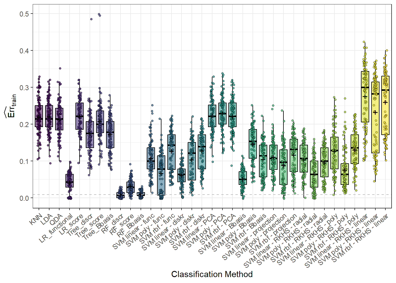
Figure 5.12: Box plots of training errors for 100 simulations separately for each classification method. The averages are marked with black \(+\) symbols.
Code
# For testing data
SIMULACE$test |>
pivot_longer(cols = methods, names_to = 'method', values_to = 'Err') |>
mutate(method = factor(method, levels = methods, labels = methods, ordered = TRUE)) |>
as.data.frame() |>
ggplot(aes(x = method, y = Err, fill = method, colour = method, alpha = method)) +
geom_boxplot(outlier.colour = "white", outlier.shape = 16, outlier.size = 0,
notch = FALSE, colour = 'black') +
theme_bw() +
labs(x = 'Classification Method',
y = expression(widehat(Err)[test])
) +
theme(legend.position = 'none',
axis.text.x = element_text(angle = 50, hjust = 1)) +
geom_jitter(position = position_jitter(0.15), alpha = 0.6, size = 0.9, pch = 21,
colour = "black") +
stat_summary(fun = "mean", geom = "point", shape = '+',
size = 3, color = "black", alpha = 0.9) +
geom_hline(yintercept = min(SIMULACE.df$Err.test),
linetype = 'dashed', colour = 'gray20', alpha = 0.8)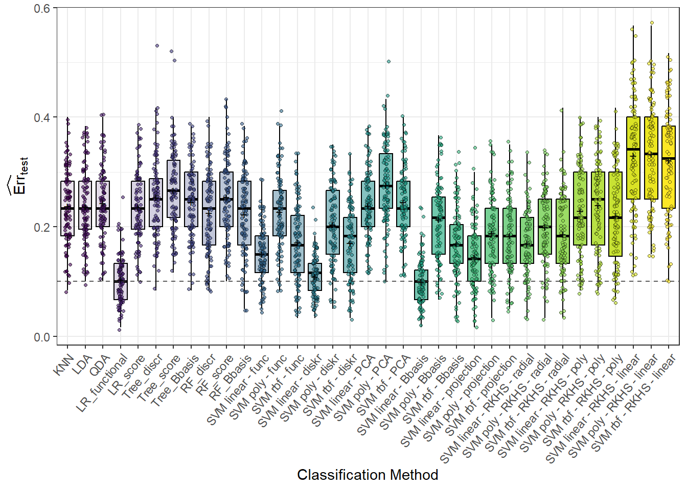
Figure 5.13: Box plots of testing errors for 100 simulations separately for each classification method. The averages are marked with black \(+\) symbols.
We would now like to formally test whether some classification methods are better than others based on the previous simulation on this data, or show that we can consider them equally successful. Due to the violation of normality assumptions, we cannot use the classic paired t-test. We will use its non-parametric alternative—the paired Wilcoxon test. However, we must be cautious in our interpretation.
Code
## [1] 0.1473608Code
## [1] 0.2346987Code
## [1] 0.002554202We are testing at the adjusted significance level \(\alpha_{adj} = 0.05 / 3 = 0.0167\).
| Median Hyperparameter Value | |
|---|---|
| KNN_K | 12.0 |
| nharm | 3.0 |
| LR_func_n_basis | 11.0 |
| SVM_d_Linear | 11.0 |
| SVM_d_Poly | 11.0 |
| SVM_d_Radial | 11.0 |
| SVM_RKHS_radial_gamma1 | 3.2 |
| SVM_RKHS_radial_gamma2 | 3.2 |
| SVM_RKHS_radial_gamma3 | 3.2 |
| SVM_RKHS_radial_d1 | 15.0 |
| SVM_RKHS_radial_d2 | 15.0 |
| SVM_RKHS_radial_d3 | 15.0 |
| SVM_RKHS_poly_p1 | 4.0 |
| SVM_RKHS_poly_p2 | 3.0 |
| SVM_RKHS_poly_p3 | 3.0 |
| SVM_RKHS_poly_d1 | 25.0 |
| SVM_RKHS_poly_d2 | 27.5 |
| SVM_RKHS_poly_d3 | 25.0 |
| SVM_RKHS_linear_d1 | 15.0 |
| SVM_RKHS_linear_d2 | 20.0 |
| SVM_RKHS_linear_d3 | 20.0 |
Code
CV_res <- CV_RESULTS |>
pivot_longer(cols = CV_RESULTS |> colnames(), names_to = 'method', values_to = 'hyperparameter') |>
mutate(method = factor(method,
levels = CV_RESULTS |> colnames(),
labels = CV_RESULTS |> colnames(), ordered = TRUE)) |>
as.data.frame()
CV_res |>
filter(method %in% c('KNN_K', 'nharm', 'LR_func_n_basis')) |>
ggplot(aes(x = hyperparameter, #y = after_stat(density),
fill = method, colour = method)) +
geom_histogram(binwidth = 1, alpha = 0.6) +
theme_bw() +
facet_grid(~method, scales = 'free') +
labs(x = 'Hyperparameter Values',
y = 'Absolute Count') +
theme(legend.position = 'none')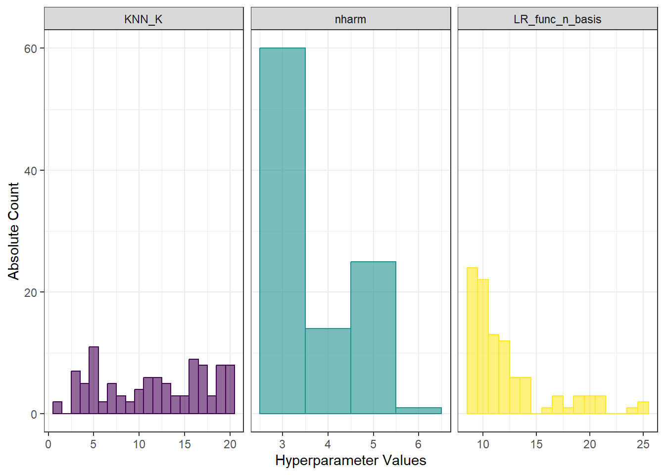
Figure 5.14: Histograms of hyperparameter values for KNN, functional logistic regression, and the number of principal components.
Code
CV_res |>
filter(method %in% c('SVM_d_Linear', 'SVM_d_Poly', 'SVM_d_Radial')) |>
ggplot(aes(x = hyperparameter, #y = after_stat(density),
fill = method, colour = method)) +
geom_histogram(binwidth = 5, alpha = 0.6) +
theme_bw() +
facet_grid(~method, scales = 'free') +
labs(x = 'Hyperparameter Values',
y = 'Absolute Count') +
theme(legend.position = 'none')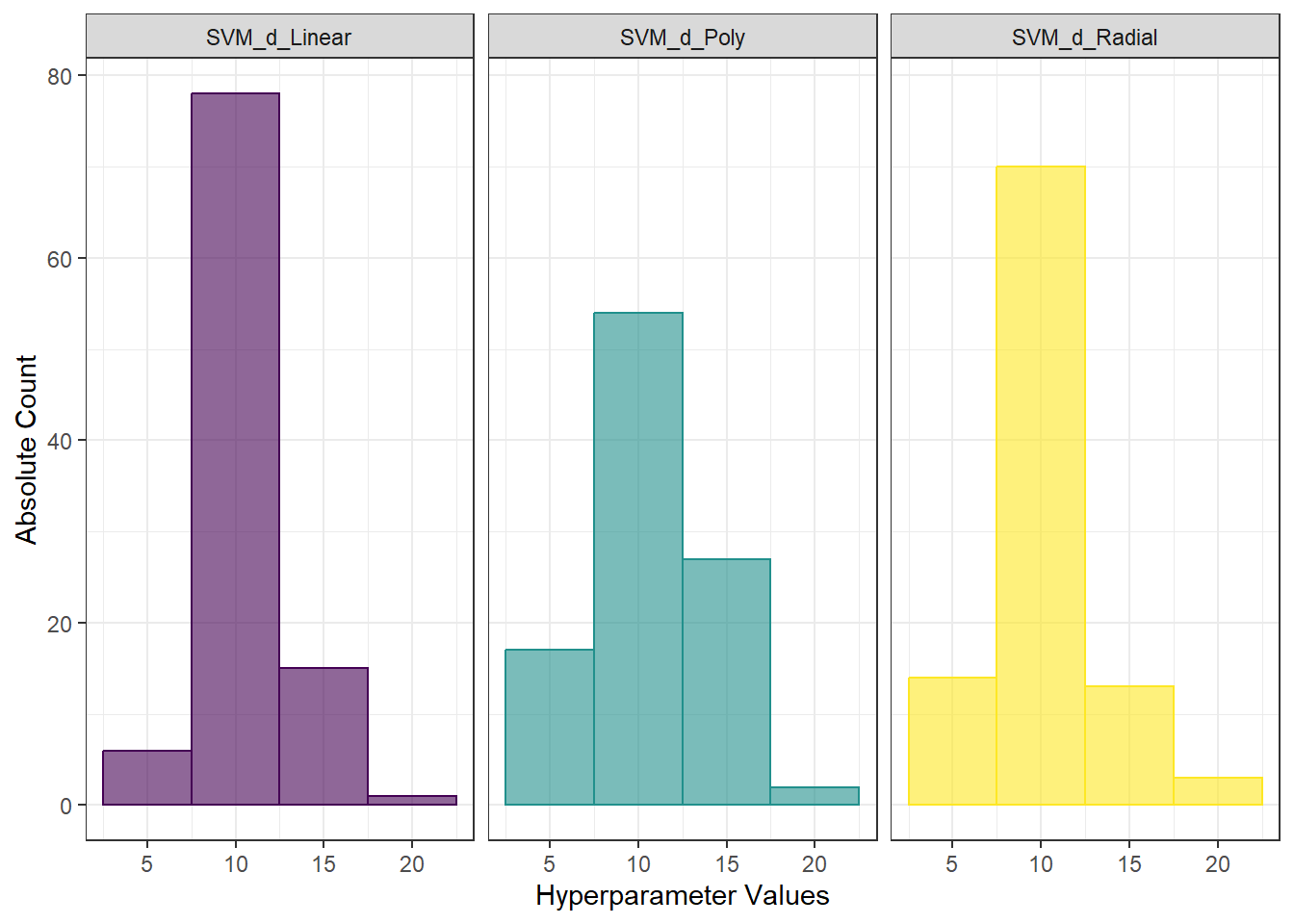
Figure 5.15: Histograms of hyperparameter values for SVM with projection onto B-spline basis.
Code
CV_res |>
filter(method %in% c('SVM_RKHS_radial_gamma1', 'SVM_RKHS_radial_gamma2',
'SVM_RKHS_radial_gamma3', 'SVM_RKHS_radial_d1',
'SVM_RKHS_radial_d2', 'SVM_RKHS_radial_d3')) |>
ggplot(aes(x = hyperparameter, #y = after_stat(density),
fill = method, colour = method)) +
geom_histogram(bins = 10, alpha = 0.6) +
theme_bw() +
facet_wrap(~method, scales = 'free', ncol = 3) +
labs(x = 'Hyperparameter Values',
y = 'Absolute Count') +
theme(legend.position = 'none')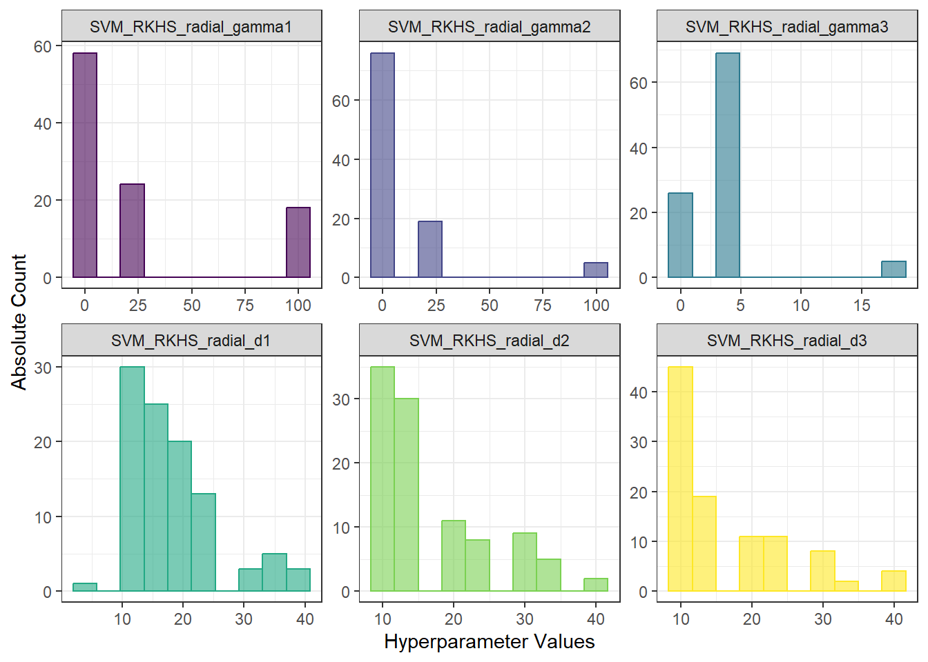
Figure 1.26: Histograms of hyperparameter values for RKHS + SVM with radial kernel.
Code
CV_res |>
filter(method %in% c('SVM_RKHS_poly_p1', 'SVM_RKHS_poly_p2',
'SVM_RKHS_poly_p3', 'SVM_RKHS_poly_d1',
'SVM_RKHS_poly_d2', 'SVM_RKHS_poly_d3')) |>
ggplot(aes(x = hyperparameter, #y = after_stat(density),
fill = method, colour = method)) +
geom_histogram(binwidth = 1, alpha = 0.6) +
theme_bw() +
facet_wrap(~method, scales = 'free', ncol = 3) +
labs(x = 'Hyperparameter Values',
y = 'Absolute Count') +
theme(legend.position = 'none')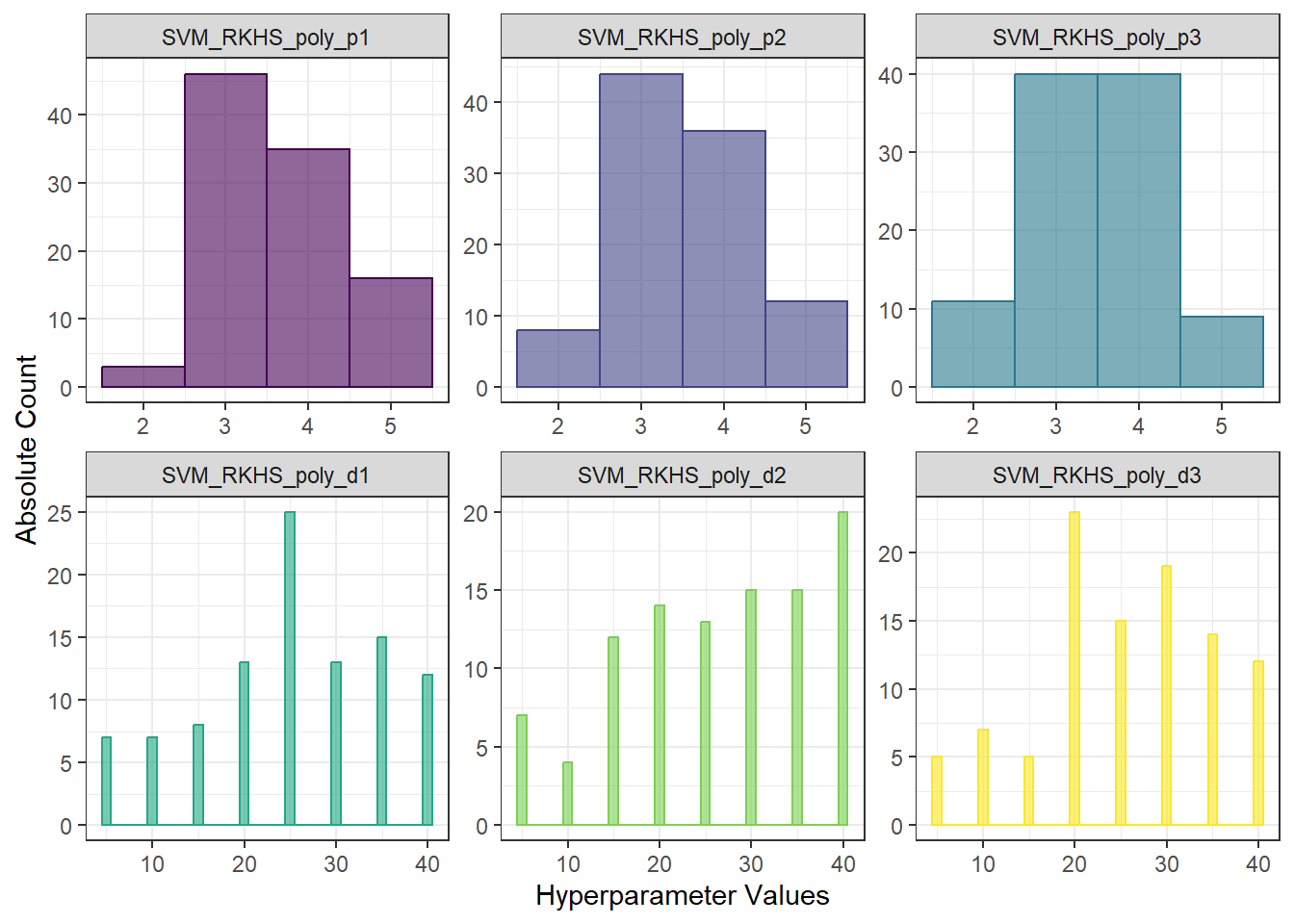
Figure 1.27: Histograms of hyperparameter values for RKHS + SVM with polynomial kernel.
Code
CV_res |>
filter(method %in% c('SVM_RKHS_linear_d1',
'SVM_RKHS_linear_d2', 'SVM_RKHS_linear_d3')) |>
ggplot(aes(x = hyperparameter, #y = after_stat(density),
fill = method, colour = method)) +
geom_histogram(binwidth = 5, alpha = 0.6) +
theme_bw() +
facet_wrap(~method, scales = 'free', ncol = 3) +
labs(x = 'Hyperparameter Values',
y = 'Absolute Count') +
theme(legend.position = 'none')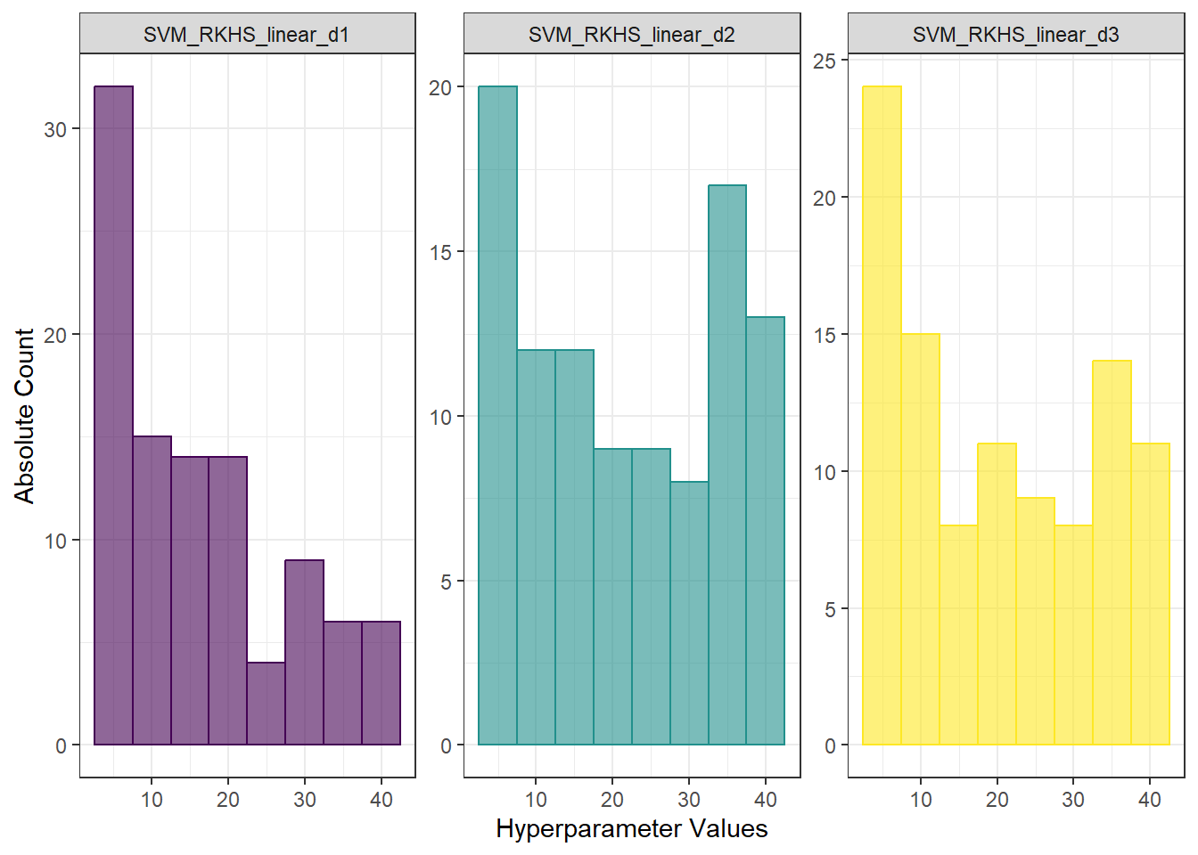
Figure 5.16: Histograms of hyperparameter values for RKHS + SVM with linear kernel.
5.2 Classification Based on the Second Derivative
In the previous section, we considered the first derivative of the curves. Now, let’s repeat the entire process with the second derivatives.
In each of the two classes, we will consider 100 observations, i.e., n = 100.
Code
We will plot the generated (yet unsmoothed) functions in color according to the class (only the first 10 observations from each class for clarity).
Code
n_curves_plot <- 10 # number of curves to be plotted from each group
DF0 <- cbind(t, X0[, 1:n_curves_plot]) |>
as.data.frame() |>
reshape(varying = 2:(n_curves_plot + 1), direction = 'long', sep = '') |>
subset(select = -id) |>
mutate(
time = time - 1,
group = 0
)
DF1 <- cbind(t, X1[, 1:n_curves_plot]) |>
as.data.frame() |>
reshape(varying = 2:(n_curves_plot + 1), direction = 'long', sep = '') |>
subset(select = -id) |>
mutate(
time = time - 1,
group = 1
)
DF <- rbind(DF0, DF1) |>
mutate(group = factor(group))
DF |> ggplot(aes(x = t, y = V, group = interaction(time, group),
colour = group)) +
geom_line(linewidth = 0.5) +
theme_bw() +
labs(x = expression(x[1]),
y = expression(x[2]),
colour = 'Class') +
scale_colour_discrete(labels=c('Y = 0', 'Y = 1'))
Figure 5.17: First 10 generated observations from each of the two classification classes. Observed data are not smoothed.
5.2.1 Smoothing of Observed Curves
Now we convert the observed discrete values (vectors of values) into functional objects, which we will work with subsequently. We will again use the B-spline basis for smoothing.
We take the entire vector t as knots; since we are considering the first derivative, we set norder = 6.
We will penalize the fourth derivative of the functions, as we now require smooth second derivatives as well.
Code
We will find a suitable value for the smoothing parameter \(\lambda > 0\) using \(GCV(\lambda)\), i.e., generalized cross-validation. We will consider the same value of \(\lambda\) for both classification groups, as we would not know in advance which value of \(\lambda\) to choose for test observations if different values were chosen for each class.
Code
# combining observations into a single matrix
XX <- cbind(X0, X1)
lambda.vect <- 10^seq(from = -4, to = -2, length.out = 50) # lambda vector
gcv <- rep(NA, length = length(lambda.vect)) # empty vector for storing GCV
for(index in 1:length(lambda.vect)) {
curv.Fdpar <- fdPar(bbasis, curv.Lfd, lambda.vect[index])
BSmooth <- smooth.basis(t, XX, curv.Fdpar) # smoothing
gcv[index] <- mean(BSmooth$gcv) # average over all observed curves
}
GCV <- data.frame(
lambda = round(log10(lambda.vect), 3),
GCV = gcv
)
# finding the minimum value
lambda.opt <- lambda.vect[which.min(gcv)]For better visualization, we will plot the course of \(GCV(\lambda)\).
Code
GCV |> ggplot(aes(x = lambda, y = GCV)) +
geom_line(linetype = 'solid', linewidth = 0.6) +
geom_point(size = 1.5) +
theme_bw() +
labs(x = bquote(paste(log[10](lambda), ' ; ',
lambda[optimal] == .(round(lambda.opt, 4)))),
y = expression(GCV(lambda))) +
geom_point(aes(x = log10(lambda.opt), y = min(gcv)), colour = 'red', size = 2.5)## Warning in geom_point(aes(x = log10(lambda.opt), y = min(gcv)), colour = "red", : All aesthetics have length 1, but the data has 50 rows.
## ℹ Please consider using `annotate()` or provide this layer with data containing
## a single row.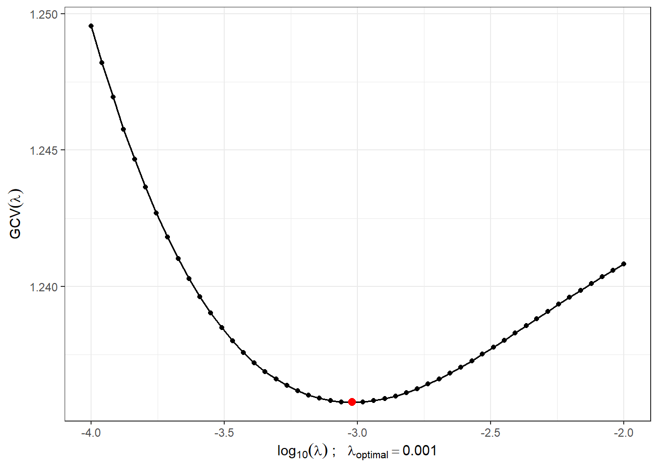
Figure 5.18: Course of \(GCV(\lambda)\) for the chosen vector \(\boldsymbol\lambda\). Values on the \(x\) axis are displayed on a logarithmic scale. The optimal value of the smoothing parameter \(\lambda_{optimal}\) is shown in red.
With this optimal choice of the smoothing parameter \(\lambda\), we will now smooth all functions and again graphically illustrate the first 10 observed curves from each classification class.
Code
curv.fdPar <- fdPar(bbasis, curv.Lfd, lambda.opt)
BSmooth <- smooth.basis(t, XX, curv.fdPar)
XXfd <- BSmooth$fd
fdobjSmootheval <- eval.fd(fdobj = XXfd, evalarg = t)
DF$Vsmooth <- c(fdobjSmootheval[, c(1 : n_curves_plot,
(n + 1) : (n + n_curves_plot))])
DF |> ggplot(aes(x = t, y = Vsmooth, group = interaction(time, group),
colour = group)) +
geom_line(linewidth = 0.75) +
theme_bw() +
labs(x = expression(x[1]),
y = expression(x[2]),
colour = 'Class') +
scale_colour_discrete(labels=c('Y = 0', 'Y = 1'))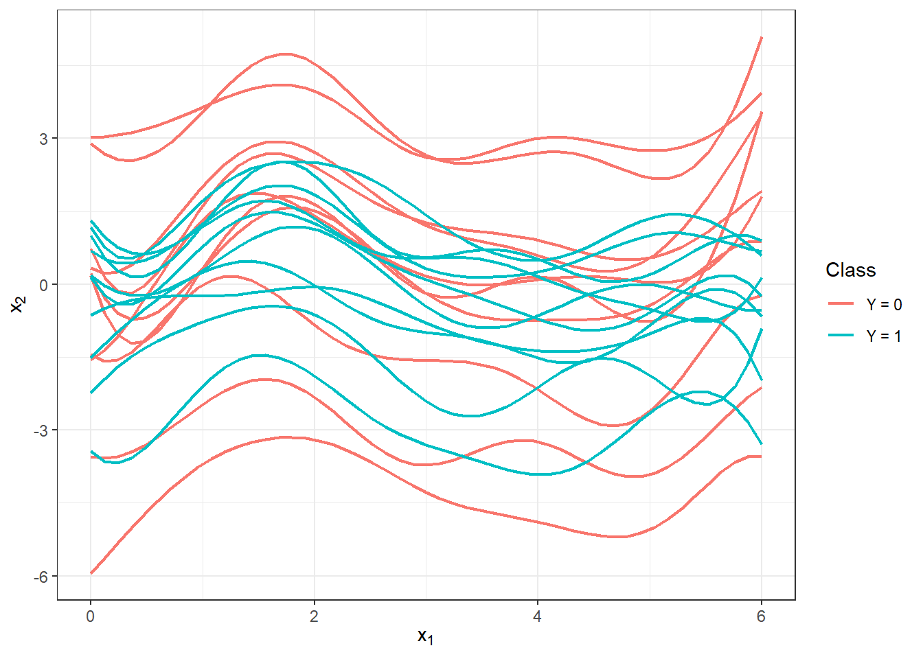
Figure 5.19: First 10 smoothed curves from each classification class.
Let’s also illustrate all curves, including the mean, separately for each class.
Code
DFsmooth <- data.frame(
t = rep(t, 2 * n),
time = rep(rep(1:n, each = length(t)), 2),
Smooth = c(fdobjSmootheval),
Mean = c(rep(apply(fdobjSmootheval[ , 1 : n], 1, mean), n),
rep(apply(fdobjSmootheval[ , (n + 1) : (2 * n)], 1, mean), n)),
group = factor(rep(c(0, 1), each = n * length(t)))
)
DFmean <- data.frame(
t = rep(t, 2),
Mean = c(apply(fdobjSmootheval[ , 1 : n], 1, mean),
apply(fdobjSmootheval[ , (n + 1) : (2 * n)], 1, mean)),
group = factor(rep(c(0, 1), each = length(t)))
)
DFsmooth |> ggplot(aes(x = t, y = Smooth, group = interaction(time, group),
colour = group)) +
geom_line(linewidth = 0.25, alpha = 0.5) +
theme_bw() +
labs(x = expression(x[1]),
y = expression(x[2]),
colour = 'Class') +
scale_colour_discrete(labels = c('Y = 0', 'Y = 1')) +
geom_line(aes(x = t, y = Mean, colour = group),
linewidth = 1.2, linetype = 'solid') +
scale_x_continuous(expand = c(0.01, 0.01)) +
#ylim(c(-1, 2)) +
scale_y_continuous(expand = c(0.01, 0.01))#, limits = c(-1, 2))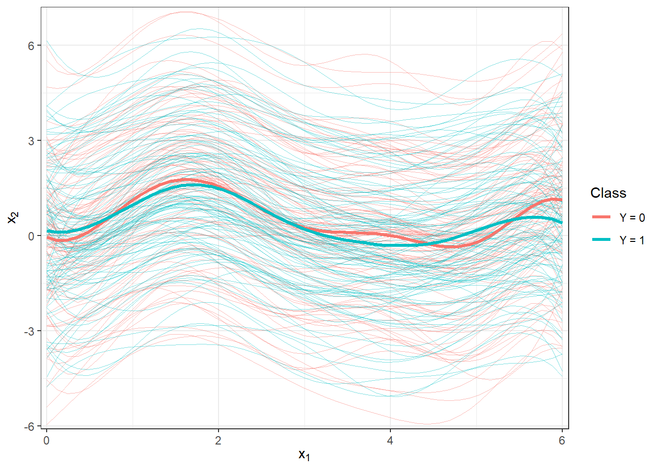
Figure 5.20: Plot of all smoothed observed curves, with curves color-coded by classification class. The mean for each class is shown with a thick line.
Code
DFsmooth <- data.frame(
t = rep(t, 2 * n),
time = rep(rep(1:n, each = length(t)), 2),
Smooth = c(fdobjSmootheval),
Mean = c(rep(apply(fdobjSmootheval[ , 1 : n], 1, mean), n),
rep(apply(fdobjSmootheval[ , (n + 1) : (2 * n)], 1, mean), n)),
group = factor(rep(c(0, 1), each = n * length(t)))
)
DFmean <- data.frame(
t = rep(t, 2),
Mean = c(apply(fdobjSmootheval[ , 1 : n], 1, mean),
apply(fdobjSmootheval[ , (n + 1) : (2 * n)], 1, mean)),
group = factor(rep(c(0, 1), each = length(t)))
)
DFsmooth |> ggplot(aes(x = t, y = Smooth, group = interaction(time, group),
colour = group)) +
geom_line(linewidth = 0.25, alpha = 0.5) +
theme_bw() +
labs(x = expression(x[1]),
y = expression(x[2]),
colour = 'Class') +
scale_colour_discrete(labels = c('Y = 0', 'Y = 1')) +
geom_line(aes(x = t, y = Mean, colour = group),
linewidth = 1.2, linetype = 'solid') +
scale_x_continuous(expand = c(0.01, 0.01)) +
#ylim(c(-1, 2)) +
scale_y_continuous(expand = c(0.01, 0.01), limits = c(-1, 2))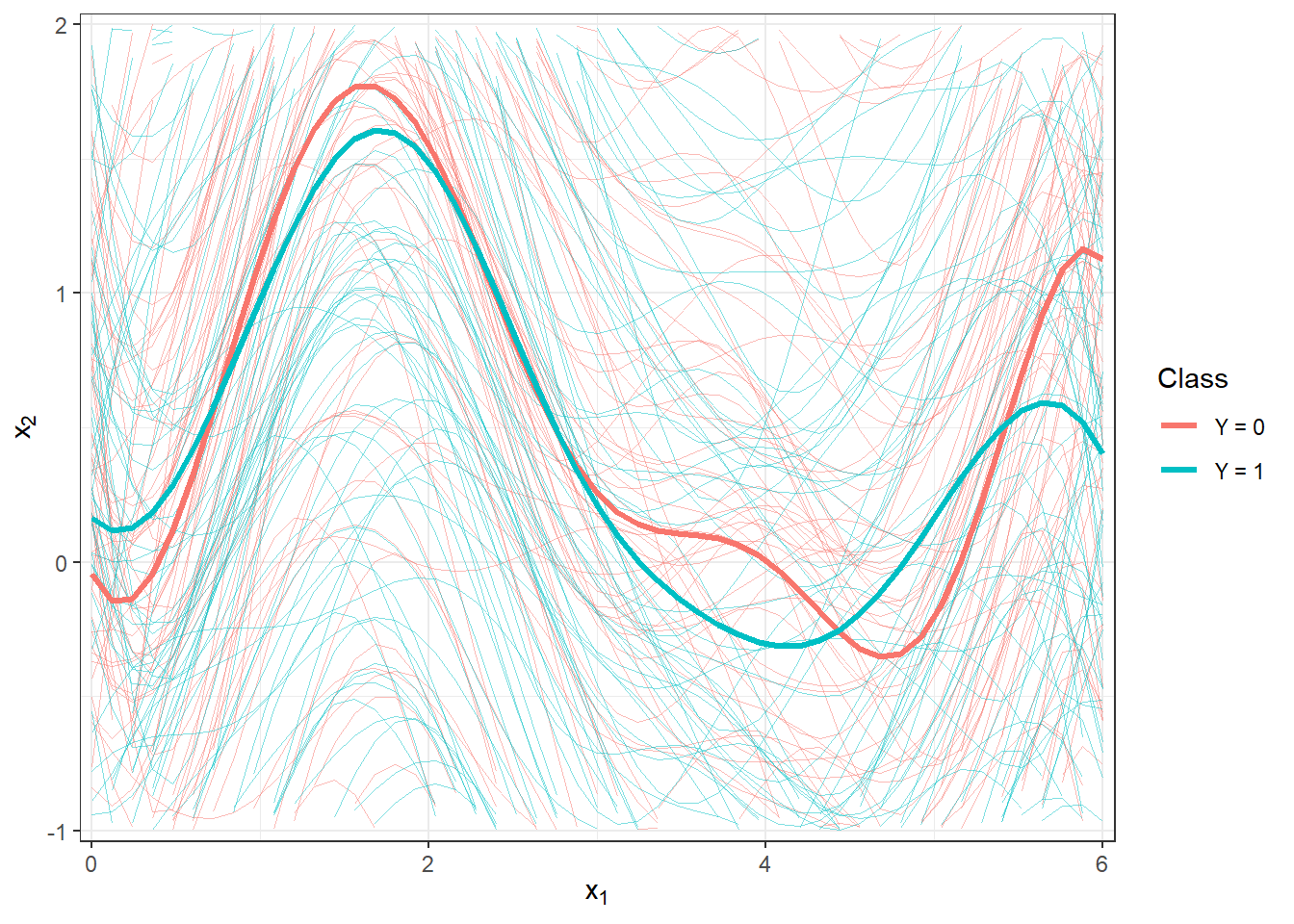
Figure 5.21: Plot of all smoothed observed curves, with curves color-coded by classification class. The mean for each class is shown with a thick line. Close-up view.
5.2.2 Derivative Calculation
To calculate the derivative for a functional object, we use the deriv.fd() function from the fda package in R. Since we aim to classify based on the second derivative, we set the argument Lfdobj = 2.
Now, let’s plot the first few derivatives for both classification classes. Notice from the figure below that the vertical shift was effectively removed through differentiation. However, this also reduced the distinctiveness between the curves, as the differences in the derivative curves between the two classes primarily occur toward the end of the interval, approximately in the range \([5, 6]\).
Code
fdobjSmootheval <- eval.fd(fdobj = XXder, evalarg = t)
DF$Vsmooth <- c(fdobjSmootheval[, c(1 : n_curves_plot,
(n + 1) : (n + n_curves_plot))])
DF |> ggplot(aes(x = t, y = Vsmooth, group = interaction(time, group),
colour = group)) +
geom_line(linewidth = 0.75) +
theme_bw() +
labs(x = expression(x[1]),
y = expression(x[2]),
colour = 'Class') +
scale_colour_discrete(labels=c('Y = 0', 'Y = 1'))
Let’s now illustrate all curves, including the mean for each class separately.
Code
abs.labs <- paste("Class:", c("$Y = 0$", "$Y = 1$"))
names(abs.labs) <- c('0', '1')
tt <- seq(min(t), max(t), length = 91)
fdobjSmootheval <- eval.fd(fdobj = XXder, evalarg = tt)
DFsmooth <- data.frame(
t = rep(tt, 2 * n),
time = rep(rep(1:n, each = length(tt)), 2),
Smooth = c(fdobjSmootheval),
group = factor(rep(c(0, 1), each = n * length(tt)))
)
DFmean <- data.frame(
t = rep(tt, 2),
Mean = c(eval.fd(fdobj = mean.fd(XXder[1:n]), evalarg = tt),
eval.fd(fdobj = mean.fd(XXder[(n + 1):(2 * n)]), evalarg = tt)),
group = factor(rep(c(0, 1), each = length(tt)))
)
DFsmooth |> ggplot(aes(x = t, y = Smooth, colour = group)) +
geom_line(aes(group = time), linewidth = 0.05, alpha = 0.5) +
theme_bw() +
labs(x = "$t$",
y = "$x_i'(t)$",
colour = 'Class') +
geom_line(data = DFmean |>
mutate(group = factor(ifelse(group == '0', '1', '0'))),
aes(x = t, y = Mean, colour = group),
colour = 'grey2', linewidth = 0.8, linetype = 'dashed') +
geom_line(data = DFmean, aes(x = t, y = Mean, colour = group),
colour = 'grey2', linewidth = 1.25, linetype = 'solid') +
scale_x_continuous(expand = c(0.01, 0.01)) +
facet_wrap(~group, labeller = labeller(group = abs.labs)) +
scale_y_continuous(expand = c(0.02, 0.02)) +
theme(legend.position = 'none',
plot.margin = unit(c(0.1, 0.1, 0.3, 0.5), "cm")) +
coord_cartesian(ylim = c(-20, 20)) +
scale_colour_manual(values = c('tomato', 'deepskyblue2'))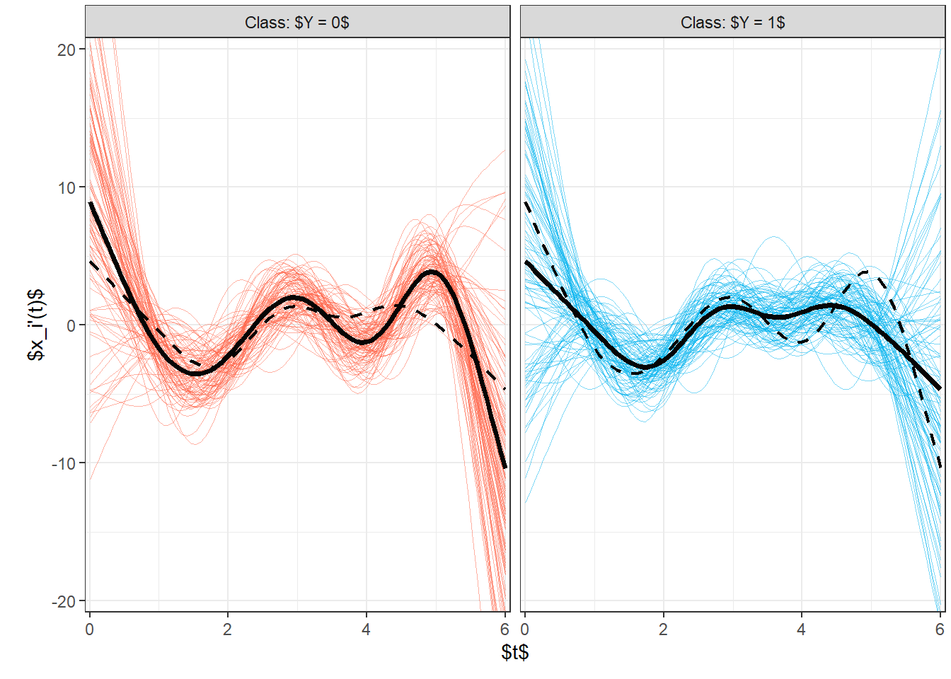
Figure 5.22: Plotting all smoothed observed curves, with color differentiation according to class. The mean for each class is shown by a black line.
Code
fdobjSmootheval <- eval.fd(fdobj = XXder, evalarg = t)
DFsmooth <- data.frame(
t = rep(t, 2 * n),
time = rep(rep(1:n, each = length(t)), 2),
Smooth = c(fdobjSmootheval),
Mean = c(rep(apply(fdobjSmootheval[ , 1 : n], 1, mean), n),
rep(apply(fdobjSmootheval[ , (n + 1) : (2 * n)], 1, mean), n)),
group = factor(rep(c(0, 1), each = n * length(t)))
)
DFmean <- data.frame(
t = rep(t, 2),
Mean = c(apply(fdobjSmootheval[ , 1 : n], 1, mean),
apply(fdobjSmootheval[ , (n + 1) : (2 * n)], 1, mean)),
group = factor(rep(c(0, 1), each = length(t)))
)
DFsmooth |> ggplot(aes(x = t, y = Smooth, group = interaction(time, group),
colour = group)) +
geom_line(linewidth = 0.25, alpha = 0.5) +
theme_bw() +
labs(x = expression(x[1]),
y = expression(x[2]),
colour = 'Class') +
scale_colour_discrete(labels = c('Y = 0', 'Y = 1')) +
geom_line(aes(x = t, y = Mean), colour = 'grey3',
linewidth = 0.7, linetype = 'dashed') +
scale_x_continuous(expand = c(0.01, 0.01)) +
scale_y_continuous(expand = c(0.01, 0.01), limits = c(-12, 10))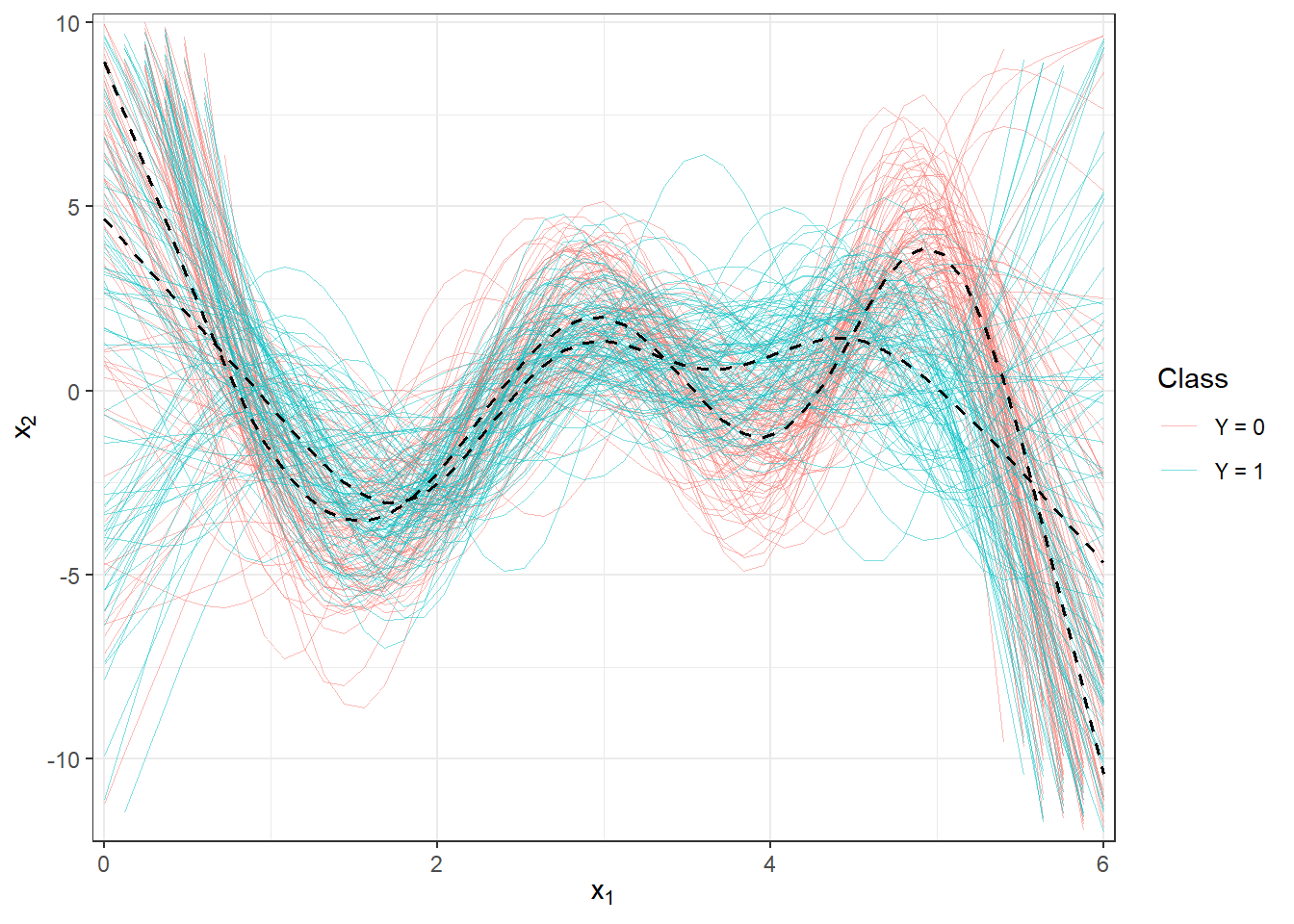
Figure 1.29: Plotting all smoothed observed curves, with color differentiation according to class. The mean for each class is shown by a black line. Zoomed view.
5.2.3 Classification of Curves
First, we will load the necessary libraries for classification.
Code
library(caTools) # for splitting into test and training sets
library(caret) # for k-fold CV
library(fda.usc) # for KNN, fLR
library(MASS) # for LDA
library(fdapace)
library(pracma)
library(refund) # for logistic regression on scores
library(nnet) # for logistic regression on scores
library(caret)
library(rpart) # decision trees
library(rattle) # visualization
library(e1071)
library(randomForest) # random forestTo compare individual classifiers, we will split the generated observations into two parts in a 70:30 ratio for training and testing (validation) sets. The training set will be used to construct the classifier, while the test set will be used to calculate the classification error and potentially other characteristics of our model. The resulting classifiers can then be compared based on these computed characteristics in terms of their classification success.
Code
Next, we will examine the representation of individual groups in the test and training portions of the data.
## Y.train
## 0 1
## 71 69## Y.test
## 0 1
## 29 31## Y.train
## 0 1
## 0.5071429 0.4928571## Y.test
## 0 1
## 0.4833333 0.51666675.2.3.1 \(K\) Nearest Neighbors
Let’s start with a non-parametric classification method, specifically the \(K\) nearest neighbors method. First, we will create the necessary objects so that we can work with them using the classif.knn() function from the fda.usc library.
Now we can define the model and look at its classification success. The last question remains how to choose the optimal number of neighbors \(K\). We could choose this number as the value of \(K\) that results in the minimum error rate on the training data. However, this could lead to overfitting the model, so we will use cross-validation. Given the computational complexity and size of the dataset, we will opt for \(k\)-fold CV; we will choose a value of \(k = 10\).
Code
# model for all training data for K = 1, 2, ..., sqrt(n_train)
neighb.model <- classif.knn(group = y.train,
                            fdataobj = x.train,
                            knn = c(1:round(sqrt(length(y.train)))))

# summary(neighb.model) # summary of the model
# plot(neighb.model$gcv, pch = 16) # plot GCV dependence on the number of neighbors K
# neighb.model$max.prob # maximum accuracy
(K.opt <- neighb.model$h.opt) # optimal value of K
## [1] 12Let’s proceed with the previous procedure for the training data, which we will split into \(k\) parts and repeat this code \(k\) times.
Code
k_cv <- 10 # k-fold CV
neighbours <- c(1:(2 * ceiling(sqrt(length(y.train))))) # number of neighbors

# split training data into k parts
folds <- createMultiFolds(X.train$fdnames$reps, k = k_cv, time = 1)

# empty matrix to store the results
# columns will contain accuracy values for the corresponding part of the training set
# rows will contain values for the given number of neighbors K
CV.results <- matrix(NA, nrow = length(neighbours), ncol = k_cv)

for (index in 1:k_cv) {
  # define the current index set
  fold <- folds[[index]]

  x.train.cv <- subset(X.train, c(1:length(X.train$fdnames$reps)) %in% fold) |>
    fdata()
  y.train.cv <- subset(Y.train, c(1:length(X.train$fdnames$reps)) %in% fold) |>
    factor() |> as.numeric()

  x.test.cv <- subset(X.train, !c(1:length(X.train$fdnames$reps)) %in% fold) |>
    fdata()
  y.test.cv <- subset(Y.train, !c(1:length(X.train$fdnames$reps)) %in% fold) |>
    factor() |> as.numeric()

  # iterate over each part ... repeat k times
  for(neighbour in neighbours) {
    # model for specific choice of K
    neighb.model <- classif.knn(group = y.train.cv,
                              fdataobj = x.train.cv,
                              knn = neighbour)
    # predictions on validation set
    model.neighb.predict <- predict(neighb.model,
                                    new.fdataobj = x.test.cv)
    # accuracy on validation set
    accuracy <- table(y.test.cv, model.neighb.predict) |>
      prop.table() |> diag() |> sum()

    # store accuracy in the position for given K and fold
    CV.results[neighbour, index] <- accuracy
  }
}

# compute average accuracies for individual K across folds
CV.results <- apply(CV.results, 1, mean)
K.opt <- which.max(CV.results)
presnost.opt.cv <- max(CV.results)
# CV.results
We can see that the best value for the parameter \(K\) is 12, with an error rate calculated using 10-fold CV of 0.1617.
For clarity, let’s also plot the validation error rate as a function of the number of neighbors \(K\).
Code
CV.results <- data.frame(K = neighbours, CV = CV.results)
CV.results |> ggplot(aes(x = K, y = 1 - CV)) +
  geom_line(linetype = 'dashed', colour = 'grey') +
  geom_point(size = 1.5) +
  geom_point(aes(x = K.opt, y = 1 - presnost.opt.cv), colour = 'red', size = 2) +
  theme_bw() +
  labs(x = bquote(paste(K, ' ;   ',
                        K[optimal] == .(K.opt))),
       y = 'Validation Error Rate') +
  scale_x_continuous(breaks = neighbours)
## Warning in geom_point(aes(x = K.opt, y = 1 - presnost.opt.cv), colour = "red", : All aesthetics have length 1, but the data has 24 rows.
## ℹ Please consider using `annotate()` or provide this layer with data containing
## a single row.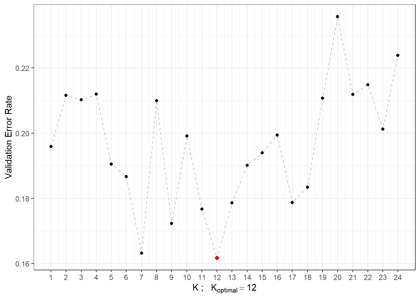
Figure 5.23: Dependency of validation error rate on the value of \(K\), i.e., on the number of neighbors.
Now that we have determined the optimal value of the parameter \(K\), we can build the final model.
Code
neighb.model <- classif.knn(group = y.train, fdataobj = x.train, knn = K.opt)

# predictions
model.neighb.predict <- predict(neighb.model,
                                new.fdataobj = fdata(X.test))

# summary(neighb.model)

# accuracy on test data
accuracy <- table(as.numeric(factor(Y.test)), model.neighb.predict) |>
  prop.table() |>
  diag() |>
  sum()
# error rate
# 1 - accuracy
Thus, the error rate of the model constructed using the \(K\)-nearest neighbors method with the optimal choice of \(K_{optimal}\) equal to 12, determined by cross-validation, is 0.15 on the training data and 0.15 on the test data.
To compare different models, we can use both types of error rates, which we will store in a table for clarity.
5.2.3.2 Linear Discriminant Analysis
As the second method for constructing a classifier, we will consider Linear Discriminant Analysis (LDA). Since this method cannot be applied to functional data, we must first discretize the data, which we will do using Functional Principal Component Analysis (FPCA). We will then perform the classification algorithm on the scores of the first \(p\) principal components. We will choose the number of components \(p\) such that the first \(p\) principal components together explain at least 90% of the variability in the data.
First, let’s perform the functional principal component analysis and determine the number \(p\).
Code
# principal component analysis
data.PCA <- pca.fd(X.train, nharm = 10) # nharm - maximum number of PCs
nharm <- which(cumsum(data.PCA$varprop) >= 0.9)[1] # determine p
if(nharm == 1) nharm <- 2

data.PCA <- pca.fd(X.train, nharm = nharm)
data.PCA.train <- as.data.frame(data.PCA$scores) # scores of the first p PCs
data.PCA.train$Y <- factor(Y.train) # class membership
In this particular case, we took the number of principal components as \(p\) = 3, which together explain 90.88 % of the variability in the data. The first principal component explains 45.83 % and the second 36.91 % of the variability. We can graphically display the scores of the first two principal components, color-coded according to class membership.
Code
data.PCA.train |> ggplot(aes(x = V1, y = V2, colour = Y)) +
  geom_point(size = 1.5) +
  labs(x = paste('1st Principal Component (explained variability',
                 round(100 * data.PCA$varprop[1], 2), '%)'),
       y = paste('2nd Principal Component (',
                 round(100 * data.PCA$varprop[2], 2), '%)'),
       colour = 'Group') +
  scale_colour_discrete(labels = c('Y = 0', 'Y = 1')) +
  theme_bw()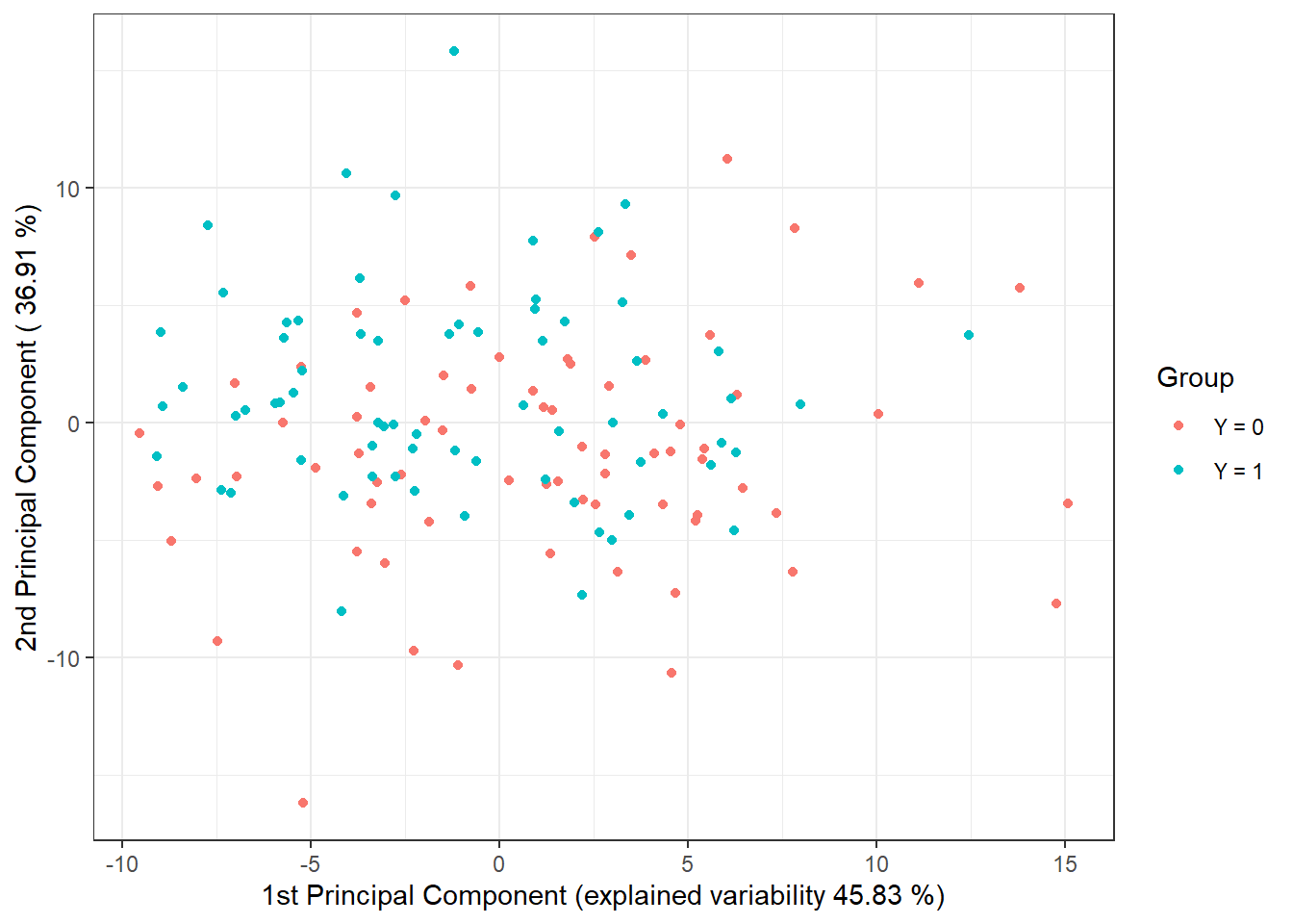
Figure 5.24: Scores of the first two principal components for the training data. Points are color-coded according to class membership.
To determine the classification accuracy on the test data, we need to calculate the scores for the first 3 principal components for the test data. These scores are determined using the formula:
\[ \xi_{i, j} = \int \left( X_i(t) - \mu(t)\right) \cdot \rho_j(t)\text{ dt}, \]
where \(\mu(t)\) is the mean function and \(\rho_j(t)\) is the eigenfunction (functional principal component).
Code
# compute scores for test functions
scores <- matrix(NA, ncol = nharm, nrow = length(Y.test)) # empty matrix

for(k in 1:dim(scores)[1]) {
  xfd = X.test[k] - data.PCA$meanfd[1] # k-th observation - mean function
  scores[k, ] = inprod(xfd, data.PCA$harmonics)
  # scalar product of residuals and eigenfunctions (functional principal components)
}

data.PCA.test <- as.data.frame(scores)
data.PCA.test$Y <- factor(Y.test)
colnames(data.PCA.test) <- colnames(data.PCA.train)
Now we can construct the classifier on the training portion of the data.
Code
# model
clf.LDA <- lda(Y ~ ., data = data.PCA.train)

# accuracy on training data
predictions.train <- predict(clf.LDA, newdata = data.PCA.train)
accuracy.train <- table(data.PCA.train$Y, predictions.train$class) |>
  prop.table() |> diag() |> sum()

# accuracy on test data
predictions.test <- predict(clf.LDA, newdata = data.PCA.test)
accuracy.test <- table(data.PCA.test$Y, predictions.test$class) |>
  prop.table() |> diag() |> sum()
We have calculated the error rate of the classifier on the training (13.57 %) and on the test data (18.33 %).
To visually represent the method, we can indicate the decision boundary in the plot of the scores of the first two principal components. We will compute this boundary on a dense grid of points and display it using the geom_contour() function.
Code
# add decision boundary
np <- 1001 # number of grid points
# x-axis ... 1st PC
nd.x <- seq(from = min(data.PCA.train$V1),
            to = max(data.PCA.train$V1), length.out = np)
# y-axis ... 2nd PC
nd.y <- seq(from = min(data.PCA.train$V2),
            to = max(data.PCA.train$V2), length.out = np)
# case for 2 PCs ... p = 2
nd <- expand.grid(V1 = nd.x, V2 = nd.y)
# if p = 3
if(dim(data.PCA.train)[2] == 4) {
  nd <- expand.grid(V1 = nd.x, V2 = nd.y, V3 = data.PCA.train$V3[1])}
# if p = 4
if(dim(data.PCA.train)[2] == 5) {
  nd <- expand.grid(V1 = nd.x, V2 = nd.y, V3 = data.PCA.train$V3[1],
                    V4 = data.PCA.train$V4[1])}
# if p = 5
if(dim(data.PCA.train)[2] == 6) {
  nd <- expand.grid(V1 = nd.x, V2 = nd.y, V3 = data.PCA.train$V3[1],
                    V4 = data.PCA.train$V4[1], V5 = data.PCA.train$V5[1])}

# add Y = 0, 1
nd <- nd |> mutate(prd = as.numeric(predict(clf.LDA, newdata = nd)$class))

data.PCA.train |> ggplot(aes(x = V1, y = V2, colour = Y)) +
  geom_point(size = 1.5) +
  labs(x = paste('1st Principal Component (explained variability',
                 round(100 * data.PCA$varprop[1], 2), '%)'),
       y = paste('2nd Principal Component (',
                 round(100 * data.PCA$varprop[2], 2), '%)'),
       colour = 'Group') +
  scale_colour_discrete(labels = c('Y = 0', 'Y = 1')) +
  theme_bw() +
  geom_contour(data = nd, aes(x = V1, y = V2, z = prd), colour = 'black')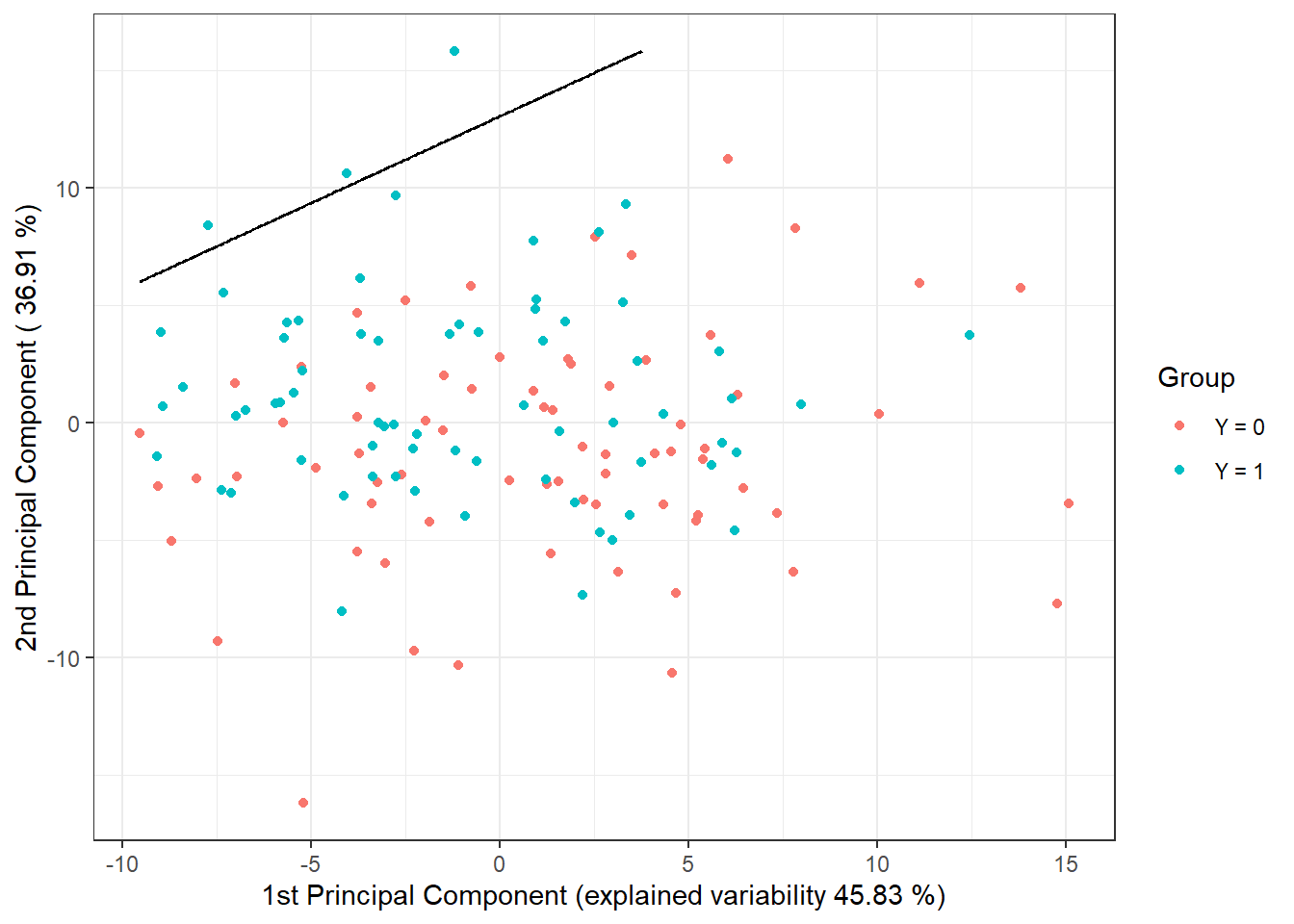
Figure 5.25: Scores of the first two principal components, color-coded according to class membership. The decision boundary (line in the plane of the first two principal components) between the classes constructed using LDA is marked in black.
We see that the decision boundary is a line, a linear function in the 2D space, which is indeed what we expected from LDA. Finally, we will add the error rates to the summary table.
5.2.3.3 Quadratic Discriminant Analysis
Next, we will construct a classifier using Quadratic Discriminant Analysis (QDA). This is an analogous case to LDA, with the difference that we now allow for different covariance matrices for each of the classes from which the corresponding scores are drawn. This relaxed assumption of equal covariance matrices leads to a quadratic boundary between the classes.
In R, we perform QDA similarly to how we did LDA in the previous section. We will compute the scores for the training and test functions using the results from the functional Principal Component Analysis (PCA) obtained earlier.
Thus, we can proceed directly to constructing the classifier using the qda() function. We will then calculate the accuracy of the classifier on both test and training data.
Code
# model
clf.QDA <- qda(Y ~ ., data = data.PCA.train)

# accuracy on training data
predictions.train <- predict(clf.QDA, newdata = data.PCA.train)
accuracy.train <- table(data.PCA.train$Y, predictions.train$class) |>
  prop.table() |> diag() |> sum()

# accuracy on test data
predictions.test <- predict(clf.QDA, newdata = data.PCA.test)
accuracy.test <- table(data.PCA.test$Y, predictions.test$class) |>
  prop.table() |> diag() |> sum()
We have calculated the error rate of the classifier on the training (14.29 %) and test data (15 %).
To visually represent the method, we can indicate the decision boundary in the plot of the scores of the first two principal components. We will compute this boundary on a dense grid of points and display it using the geom_contour() function, just like in the case of LDA.
Code
nd <- nd |> mutate(prd = as.numeric(predict(clf.QDA, newdata = nd)$class))

data.PCA.train |> ggplot(aes(x = V1, y = V2, colour = Y)) +
  geom_point(size = 1.5) +
  labs(x = paste('1st Principal Component (explained variability',
                 round(100 * data.PCA$varprop[1], 2), '%)'),
       y = paste('2nd Principal Component (',
                 round(100 * data.PCA$varprop[2], 2), '%)'),
       colour = 'Group') +
  scale_colour_discrete(labels = c('Y = 0', 'Y = 1')) +
  theme_bw() +
  geom_contour(data = nd, aes(x = V1, y = V2, z = prd), colour = 'black')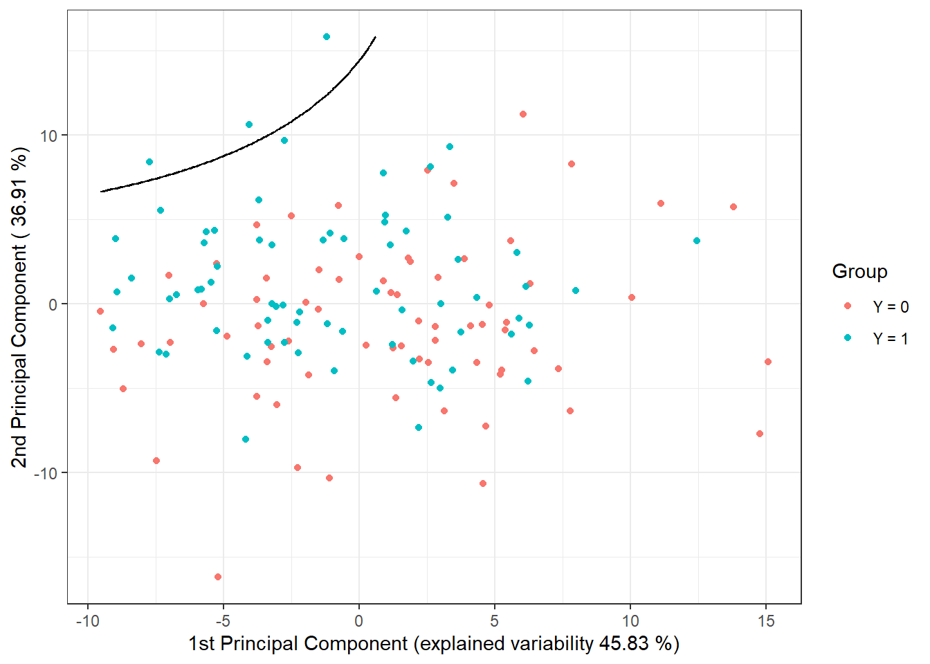
Figure 5.26: Scores of the first two principal components, color-coded according to class membership. The decision boundary (parabola in the plane of the first two principal components) between the classes constructed using QDA is marked in black.
Notice that the decision boundary between the classification classes is now a parabola.
Finally, we will add the error rates to the summary table.
5.2.3.4 Logistic Regression
We can perform logistic regression in two ways. First, we can use the functional analogue of classical logistic regression, and second, we can apply classical multivariate logistic regression on the scores of the first \(p\) principal components.
5.2.3.4.1 Functional Logistic Regression
Analogous to the case with finite-dimensional input data, we consider the logistic model in the form:
\[ g\left(\mathbb E [Y|X = x]\right) = \eta (x) = g(\pi(x)) = \alpha + \int \beta(t)\cdot x(t) \text d t, \]
where \(\eta(x)\) is a linear predictor taking values in the interval \((-\infty, \infty)\), \(g(\cdot)\) is the link function (in the case of logistic regression, this is the logit function \(g: (0,1) \rightarrow \mathbb R,\ g(p) = \ln\frac{p}{1-p}\)), and \(\pi(x)\) is the conditional probability:
\[ \pi(x) = \text{Pr}(Y = 1 | X = x) = g^{-1}(\eta(x)) = \frac{\text e^{\alpha + \int \beta(t)\cdot x(t) \text d t}}{1 + \text e^{\alpha + \int \beta(t)\cdot x(t) \text d t}}, \]
where \(\alpha\) is a constant and \(\beta(t) \in L^2[a, b]\) is a parametric function. Our goal is to estimate this parametric function.
For functional logistic regression, we will use the fregre.glm() function from the fda.usc package. First, we will create suitable objects for the classifier construction.
Code
# create suitable objects
x.train <- fdata(X.train)
y.train <- as.numeric(Y.train)
# points at which the functions are evaluated
tt <- x.train[["argvals"]]
dataf <- as.data.frame(y.train)
colnames(dataf) <- "Y"
# B-spline basis
# basis1 <- X.train$basis
nbasis.x <- 50
basis1 <- create.bspline.basis(rangeval = rangeval,
norder = norder,
nbasis = nbasis.x)To estimate the parametric function \(\beta(t)\), we need to express it in some basis representation, in our case, a B-spline basis. However, we need to determine a suitable number of basis functions. We could determine this based on the error rate on the training data, but this would lead to a preference for selecting a large number of bases, resulting in overfitting.
Let us illustrate this with the following case. For each number of bases \(n_{basis} \in \{4, 5, \dots, 50\}\), we will train the model on the training data, determine the error rate on the training data, and also calculate the error rate on the test data. We must remember that we cannot use the same data for estimating the test error rate, as this would underestimate the error rate.
Code
n.basis.max <- 50
n.basis <- 4:n.basis.max
pred.baz <- matrix(NA, nrow = length(n.basis), ncol = 2,
                   dimnames = list(n.basis, c('Err.train', 'Err.test')))

for (i in n.basis) {
  # basis for betas
  basis2 <- create.bspline.basis(rangeval = range(tt), nbasis = i)
  # formula
  f <- Y ~ x
  # basis for x and betas
  basis.x <- list("x" = basis1) # smoothed data
  basis.b <- list("x" = basis2)
  # input data for the model
  ldata <- list("df" = dataf, "x" = x.train)
  # binomial model ... logistic regression model
  model.glm <- fregre.glm(f, family = binomial(), data = ldata,
                          basis.x = basis.x, basis.b = basis.b)

  # accuracy on training data
  predictions.train <- predict(model.glm, newx = ldata)
  predictions.train <- data.frame(Y.pred = ifelse(predictions.train < 1/2, 0, 1))
  accuracy.train <- table(Y.train, predictions.train$Y.pred) |>
    prop.table() |> diag() |> sum()

  # accuracy on test data
  newldata = list("df" = as.data.frame(Y.test), "x" = fdata(X.test))
  predictions.test <- predict(model.glm, newx = newldata)
  predictions.test <- data.frame(Y.pred = ifelse(predictions.test < 1/2, 0, 1))
  accuracy.test <- table(Y.test, predictions.test$Y.pred) |>
    prop.table() |> diag() |> sum()

  # insert into the matrix
  pred.baz[as.character(i), ] <- 1 - c(accuracy.train, accuracy.test)
}

pred.baz <- as.data.frame(pred.baz)
pred.baz$n.basis <- n.basis
Let’s visualize the trends of both training and test error rates in a graph based on the number of basis functions.
Code
n.basis.beta.opt <- pred.baz$n.basis[which.min(pred.baz$Err.test)]

pred.baz |> ggplot(aes(x = n.basis, y = Err.test)) +
  geom_line(linetype = 'dashed', colour = 'black') +
  geom_line(aes(x = n.basis, y = Err.train), colour = 'deepskyblue3',
            linetype = 'dashed', linewidth = 0.5) +
  geom_point(size = 1.5) +
  geom_point(aes(x = n.basis, y = Err.train), colour = 'deepskyblue3',
             size = 1.5) +
  geom_point(aes(x = n.basis.beta.opt, y = min(pred.baz$Err.test)),
             colour = 'red', size = 2) +
  theme_bw() +
  labs(x = bquote(paste(n[basis], ' ;   ',
                        n[optimal] == .(n.basis.beta.opt))),
        y = 'Error Rate')
## Warning: Use of `pred.baz$Err.test` is discouraged.
## ℹ Use `Err.test` instead.## Warning in geom_point(aes(x = n.basis.beta.opt, y = min(pred.baz$Err.test)), : All aesthetics have length 1, but the data has 47 rows.
## ℹ Please consider using `annotate()` or provide this layer with data containing
## a single row.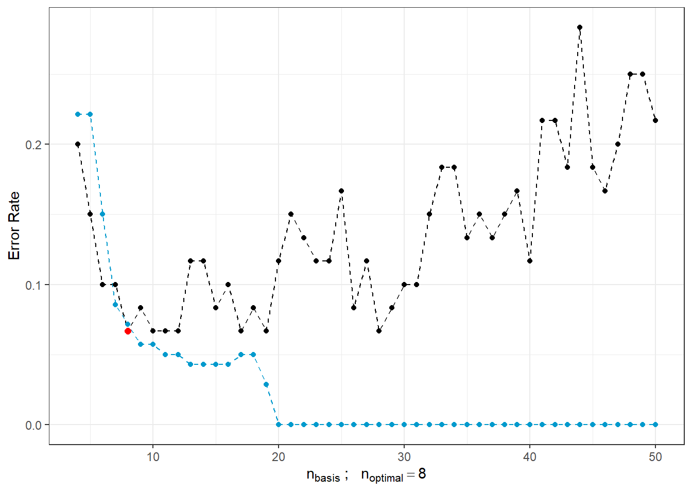
Figure 5.27: Dependence of test and training error rates on the number of basis functions for \(\beta\). The red point represents the optimal number \(n_{optimal}\) chosen as the minimum test error rate, the black line depicts the test error, and the blue dashed line illustrates the training error rate.
We see that as the number of bases for \(\beta(t)\) increases, the training error rate (represented by the blue line) tends to decrease, suggesting that we might choose large values for \(n_{basis}\) based solely on it. In contrast, the optimal choice based on the test error rate is \(n\) equal to 8, which is significantly smaller than 50. Conversely, as \(n\) increases, the test error rate rises, indicating overfitting of the model.
For these reasons, we will use 10-fold cross-validation to determine the optimal number of basis functions for \(\beta(t)\). The maximum number of basis functions considered is 35, as we observed that exceeding this value leads to overfitting.
Code
### 10-fold cross-validation
n.basis.max <- 35
n.basis <- 4:n.basis.max
k_cv <- 10 # k-fold CV
# divide the training data into k parts
folds <- createMultiFolds(X.train$fdnames$reps, k = k_cv, time = 1)
## elements that do not change during the loop
# points at which the functions are evaluated
tt <- x.train[["argvals"]]
rangeval <- range(tt)
# B-spline basis
# basis1 <- X.train$basis
# formula
f <- Y ~ x
# basis for x
basis.x <- list("x" = basis1)
# empty matrix to store results
# columns will contain accuracy values for the respective training subset
# rows will contain values for the respective number of bases
CV.results <- matrix(NA, nrow = length(n.basis), ncol = k_cv,
dimnames = list(n.basis, 1:k_cv))Now that we have everything prepared, we will calculate the error rates for each of the ten subsets of the training set. Subsequently, we will determine the average error and take the argument of the minimum validation error as the optimal \(n\).
Code
for (index in 1:k_cv) {
  # define the index set
  fold <- folds[[index]]

  x.train.cv <- subset(X.train, c(1:length(X.train$fdnames$reps)) %in% fold) |>
    fdata()
  y.train.cv <- subset(Y.train, c(1:length(X.train$fdnames$reps)) %in% fold) |>
    as.numeric()

  x.test.cv <- subset(X.train, !c(1:length(X.train$fdnames$reps)) %in% fold) |>
    fdata()
  y.test.cv <- subset(Y.train, !c(1:length(X.train$fdnames$reps)) %in% fold) |>
    as.numeric()

  dataf <- as.data.frame(y.train.cv)
  colnames(dataf) <- "Y"

  for (i in n.basis) {
    # basis for betas
    basis2 <- create.bspline.basis(rangeval = rangeval, nbasis = i)

    basis.b <- list("x" = basis2)
    # input data for the model
    ldata <- list("df" = dataf, "x" = x.train.cv)
    # binomial model ... logistic regression model
    model.glm <- fregre.glm(f, family = binomial(), data = ldata,
                            basis.x = basis.x, basis.b = basis.b)

    # accuracy on the validation subset
    newldata = list("df" = as.data.frame(y.test.cv), "x" = x.test.cv)
    predictions.valid <- predict(model.glm, newx = newldata)
    predictions.valid <- data.frame(Y.pred = ifelse(predictions.valid < 1/2, 0, 1))
    accuracy.valid <- table(y.test.cv, predictions.valid$Y.pred) |>
      prop.table() |> diag() |> sum()

    # insert into the matrix
    CV.results[as.character(i), as.character(index)] <- accuracy.valid
  }
}

# calculate average accuracies for each n across folds
CV.results <- apply(CV.results, 1, mean)
n.basis.opt <- n.basis[which.max(CV.results)]
presnost.opt.cv <- max(CV.results)
# CV.results
Let’s plot the validation error rates, highlighting the optimal value of \(n_{optimal}\), which is 15, with a validation error rate of 0.1026.
Code
CV.results <- data.frame(n.basis = n.basis, CV = CV.results)
CV.results |> ggplot(aes(x = n.basis, y = 1 - CV)) +
  geom_line(linetype = 'dashed', colour = 'grey') +
  geom_point(size = 1.5) +
  geom_point(aes(x = n.basis.opt, y = 1 - presnost.opt.cv), colour = 'red', size = 2) +
  theme_bw() +
  labs(x = bquote(paste(n[basis], ' ;   ',
                        n[optimal] == .(n.basis.opt))),
       y = 'Validation Error Rate') +
  scale_x_continuous(breaks = n.basis)
## Warning in geom_point(aes(x = n.basis.opt, y = 1 - presnost.opt.cv), colour = "red", : All aesthetics have length 1, but the data has 32 rows.
## ℹ Please consider using `annotate()` or provide this layer with data containing
## a single row.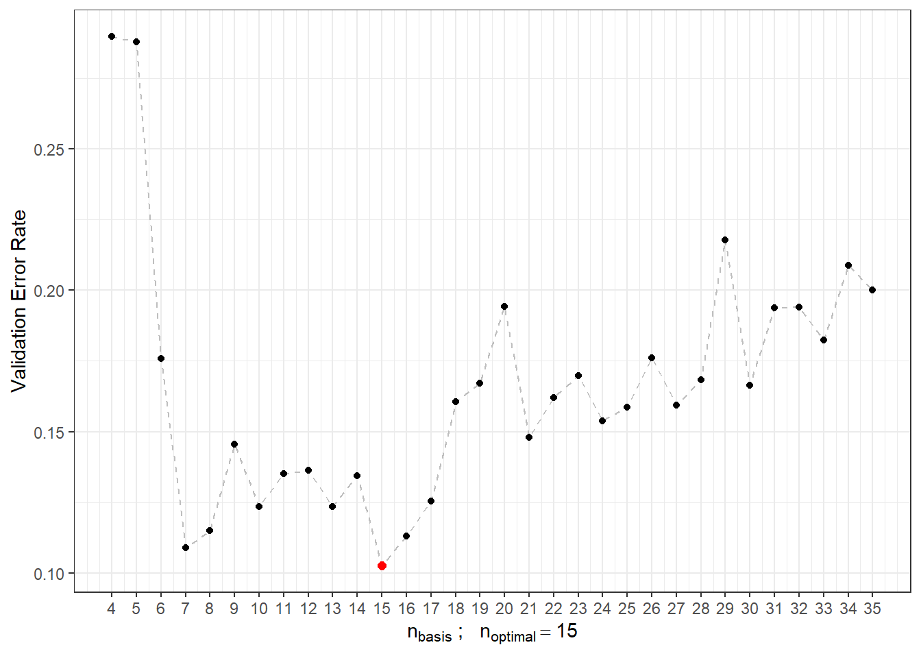
Figure 5.28: Dependence of validation error on the value of \(n_{basis}\), i.e., on the number of bases.
We can now define the final model using functional logistic regression, choosing the B-spline basis for \(\beta(t)\) with 15 bases.
Code
# optimal model
basis2 <- create.bspline.basis(rangeval = range(tt), nbasis = n.basis.opt)
f <- Y ~ x
# bases for x and betas
basis.x <- list("x" = basis1)
basis.b <- list("x" = basis2)
# input data for the model
dataf <- as.data.frame(y.train)
colnames(dataf) <- "Y"
ldata <- list("df" = dataf, "x" = x.train)
# binomial model ... logistic regression model
model.glm <- fregre.glm(f, family = binomial(), data = ldata,
                        basis.x = basis.x, basis.b = basis.b)

# accuracy on training data
predictions.train <- predict(model.glm, newx = ldata)
predictions.train <- data.frame(Y.pred = ifelse(predictions.train < 1/2, 0, 1))
presnost.train <- table(Y.train, predictions.train$Y.pred) |>
  prop.table() |> diag() |> sum()

# accuracy on test data
newldata = list("df" = as.data.frame(Y.test), "x" = fdata(X.test))
predictions.test <- predict(model.glm, newx = newldata)
predictions.test <- data.frame(Y.pred = ifelse(predictions.test < 1/2, 0, 1))
presnost.test <- table(Y.test, predictions.test$Y.pred) |>
  prop.table() |> diag() |> sum()
We have calculated the training error rate (which is 4.29 %) and the test error rate (which is 8.33 %). For better visualization, we can also plot the estimated probabilities of belonging to the classification class \(Y = 1\) on the training data against the values of the linear predictor.
Code
data.frame(
  linear.predictor = model.glm$linear.predictors,
  response = model.glm$fitted.values,
  Y = factor(y.train)
) |> ggplot(aes(x = linear.predictor, y = response, colour = Y)) +
  geom_point(size = 1.5) +
  scale_colour_discrete(labels = c('Y = 0', 'Y = 1')) +
  geom_abline(aes(slope = 0, intercept = 0.5), linetype = 'dashed') +
  theme_bw() +
  labs(x = 'Linear Predictor',
       y = 'Estimated Probability Pr(Y = 1|X = x)',
colour = 'Class') 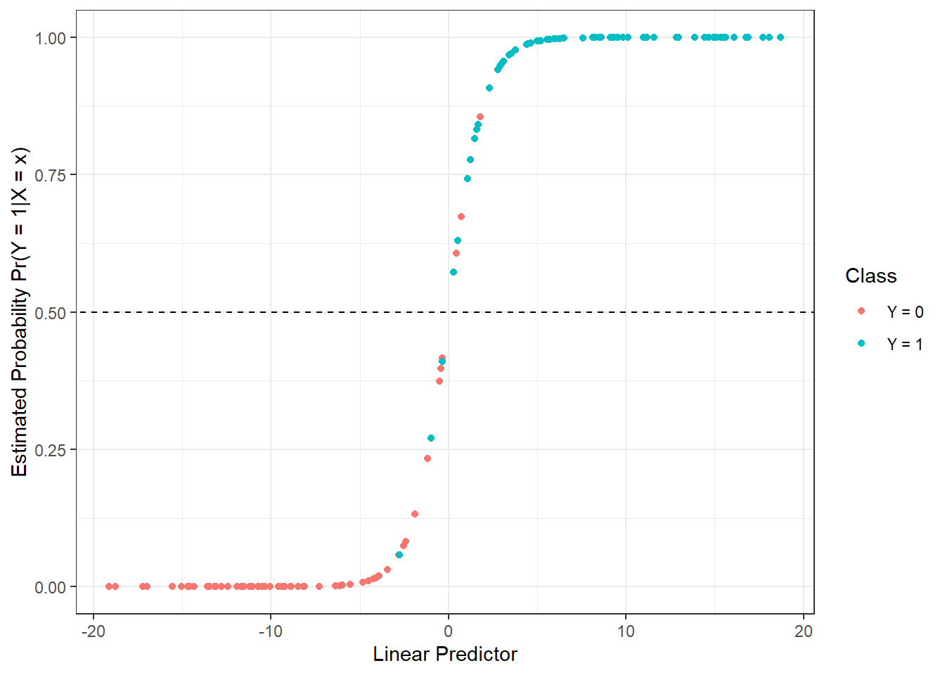
Figure 5.29: Dependence of estimated probabilities on the values of the linear predictor. Points are color-coded according to their classification class.
For informational purposes, we can also display the progression of the estimated parametric function \(\beta(t)\).
Code
t.seq <- seq(0, 6, length = 1001)
beta.seq <- eval.fd(evalarg = t.seq, fdobj = model.glm$beta.l$x)

data.frame(t = t.seq, beta = beta.seq) |>
  ggplot(aes(t, beta)) +
  geom_line() +
  theme_bw() +
  labs(x = 'Time',
       y = expression(widehat(beta)(t))) +
  theme(panel.grid.major = element_blank(), panel.grid.minor = element_blank()) +
  geom_abline(aes(slope = 0, intercept = 0), linetype = 'dashed',
linewidth = 0.5, colour = 'grey')![Plot of the estimated parametric function $\beta(t), t \in [0, 6]$.](05-Simulace_deriv2_files/figure-html/unnamed-chunk-186-1.png)
Figure 5.30: Plot of the estimated parametric function \(\beta(t), t \in [0, 6]\).
Finally, we will add the results to the summary table.
5.2.3.4.2 Logistic Regression with Principal Component Analysis
To construct this classifier, we need to perform functional principal component analysis, determine the appropriate number of components, and calculate the score values for the test data. We have already completed this in the linear discriminant analysis section, so we will use these results in the following section.
We can directly construct the logistic regression model using the glm(, family = binomial) function.
Code
# model
clf.LR <- glm(Y ~ ., data = data.PCA.train, family = binomial)

# accuracy on training data
predictions.train <- predict(clf.LR, newdata = data.PCA.train, type = 'response')
predictions.train <- ifelse(predictions.train > 0.5, 1, 0)
presnost.train <- table(data.PCA.train$Y, predictions.train) |>
  prop.table() |> diag() |> sum()

# accuracy on test data
predictions.test <- predict(clf.LR, newdata = data.PCA.test, type = 'response')
predictions.test <- ifelse(predictions.test > 0.5, 1, 0)
presnost.test <- table(data.PCA.test$Y, predictions.test) |>
  prop.table() |> diag() |> sum()
We have calculated the error rate of the classifier on the training data (13.57 %) and on the test data (18.33 %).
For graphical representation of the method, we can plot the decision boundary in the scores of the first two principal components. We will compute this boundary on a dense grid of points and display it using the geom_contour() function, just as we did in the LDA and QDA cases.
Code
nd <- nd |> mutate(prd = as.numeric(predict(clf.LR, newdata = nd,
                                            type = 'response')))
nd$prd <- ifelse(nd$prd > 0.5, 1, 0)

data.PCA.train |> ggplot(aes(x = V1, y = V2, colour = Y)) +
  geom_point(size = 1.5) +
  labs(x = paste('1st Principal Component (explained variance',
                 round(100 * data.PCA$varprop[1], 2), '%)'),
       y = paste('2nd Principal Component (',
                 round(100 * data.PCA$varprop[2], 2), '%)'),
       colour = 'Group') +
  scale_colour_discrete(labels = c('Y = 0', 'Y = 1')) +
  theme_bw() +
  geom_contour(data = nd, aes(x = V1, y = V2, z = prd), colour = 'black')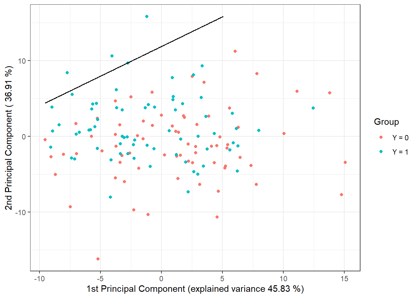
Figure 5.31: Scores of the first two principal components, color-coded according to classification class. The decision boundary (a line in the plane of the first two principal components) between classes is indicated in black, constructed using logistic regression.
Note that the decision boundary between the classification classes is now a line, similar to the case with LDA.
Finally, we will add the error rates to the summary table.
5.2.3.5 Decision Trees
In this section, we will look at a very different approach to constructing a classifier compared to methods such as LDA or logistic regression. Decision trees are a very popular tool for classification; however, like some of the previous methods, they are not directly designed for functional data. There are, however, procedures to convert functional objects into multidimensional ones, allowing us to apply decision tree algorithms. We can consider the following approaches:
An algorithm built on basis coefficients,
Utilizing principal component scores,
Discretizing the interval and evaluating the function only on a finite grid of points.
We will first focus on discretizing the interval and then compare the results with the other two approaches to constructing decision trees.
5.2.3.5.1 Interval Discretization
First, we need to define points from the interval \(I = [0, 6]\), where we will evaluate the functions. Next, we will create an object where the rows represent the individual (discretized) functions and the columns represent time. Finally, we will add a column \(Y\) containing information about the classification class and repeat the same for the test data.
Code
# sequence of points at which we will evaluate the functions
t.seq <- seq(0, 6, length = 101)

grid.data <- eval.fd(fdobj = X.train, evalarg = t.seq)
grid.data <- as.data.frame(t(grid.data)) # transpose for functions in rows
grid.data$Y <- Y.train |> factor()

grid.data.test <- eval.fd(fdobj = X.test, evalarg = t.seq)
grid.data.test <- as.data.frame(t(grid.data.test))
grid.data.test$Y <- Y.test |> factor()
Now we can construct a decision tree where all times from the vector t.seq will serve as predictors. This classification method is not susceptible to multicollinearity, so we do not need to worry about it. We will choose accuracy as the metric.
Code
# model construction
clf.tree <- train(Y ~ ., data = grid.data,
                 method = "rpart",
                 trControl = trainControl(method = "CV", number = 10),
                 metric = "Accuracy")

# accuracy on training data
predictions.train <- predict(clf.tree, newdata = grid.data)
presnost.train <- table(Y.train, predictions.train) |>
  prop.table() |> diag() |> sum()

# accuracy on test data
predictions.test <- predict(clf.tree, newdata = grid.data.test)
presnost.test <- table(Y.test, predictions.test) |>
  prop.table() |> diag() |> sum()
The error rate of the classifier on the test data is thus 15 %, and on the training data 8.57 %.
We can visualize the decision tree graphically using the fancyRpartPlot() function. We will set the colors of the nodes to reflect the previous color differentiation. This is an unpruned tree.
Code

Figure 5.32: Graphical representation of the unpruned decision tree. Blue shades represent nodes belonging to classification class 1, and red shades represent class 0.
We can also plot the final pruned decision tree.
Code
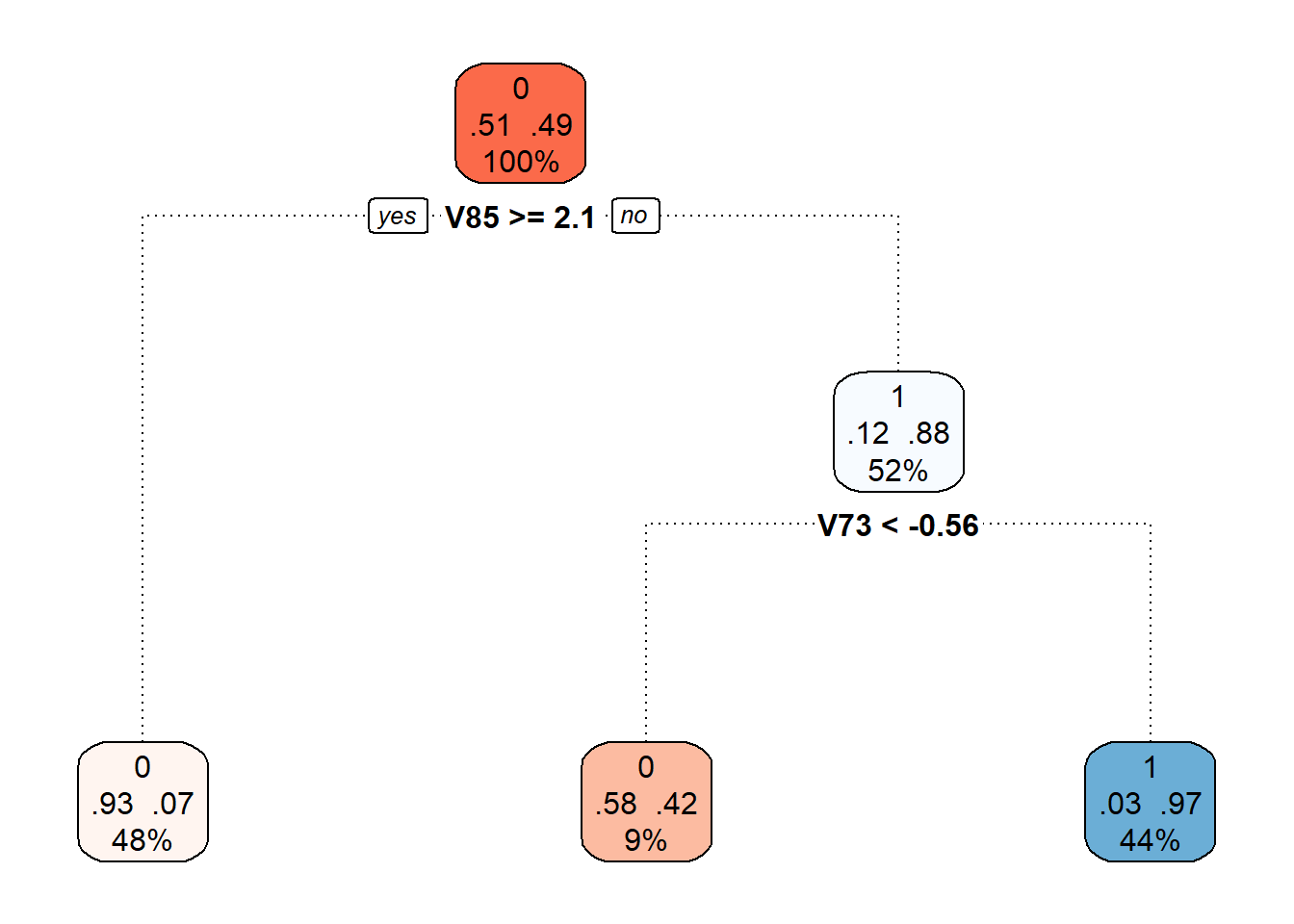
Figure 5.33: Final pruned decision tree.
Finally, we will again add the training and test error rates to the summary table.
5.2.3.5.2 Principal Component Scores
Another option for constructing a decision tree is to use principal component scores. Since we have already calculated the scores for the previous classification methods, we will utilize this knowledge and construct a decision tree based on the scores of the first 3 principal components.
Code
# model construction
clf.tree.PCA <- train(Y ~ ., data = data.PCA.train,
                 method = "rpart",
                 trControl = trainControl(method = "CV", number = 10),
                 metric = "Accuracy")

# accuracy on training data
predictions.train <- predict(clf.tree.PCA, newdata = data.PCA.train)
presnost.train <- table(Y.train, predictions.train) |>
  prop.table() |> diag() |> sum()

# accuracy on test data
predictions.test <- predict(clf.tree.PCA, newdata = data.PCA.test)
presnost.test <- table(Y.test, predictions.test) |>
  prop.table() |> diag() |> sum()
The error rate of the decision tree on the test data is thus 28.33 %, and on the training data 16.43 %.
We can visualize the decision tree constructed on the principal component scores using the fancyRpartPlot() function. We will set the colors of the nodes to reflect the previous color differentiation. This is an unpruned tree.
Code
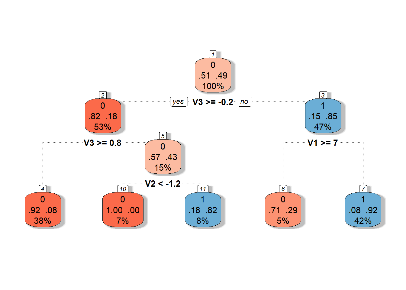
Figure 5.34: Graphical representation of the unpruned decision tree constructed on principal component scores. Blue shades represent nodes belonging to classification class 1, and red shades represent class 0.
We can also plot the final pruned decision tree.
Code
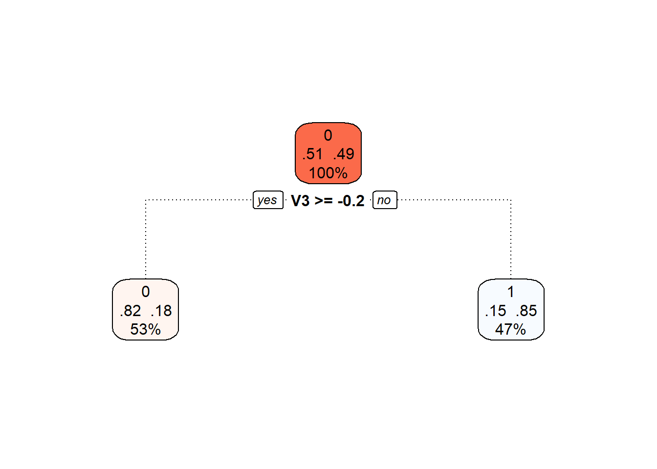
Figure 5.35: Final pruned decision tree.
Finally, we will again add the training and test error rates to the summary table.
5.2.3.5.3 Basis Coefficients
The final option we will utilize for constructing a decision tree is to use coefficients in the representation of functions in the B-spline basis.
First, let’s define the necessary datasets with the coefficients.
Code
Now we can construct the classifier.
Code
# model construction
clf.tree.Bbasis <- train(Y ~ ., data = data.Bbasis.train,
                 method = "rpart",
                 trControl = trainControl(method = "CV", number = 10),
                 metric = "Accuracy")

# accuracy on training data
predictions.train <- predict(clf.tree.Bbasis, newdata = data.Bbasis.train)
presnost.train <- table(Y.train, predictions.train) |>
  prop.table() |> diag() |> sum()

# accuracy on test data
predictions.test <- predict(clf.tree.Bbasis, newdata = data.Bbasis.test)
presnost.test <- table(Y.test, predictions.test) |>
  prop.table() |> diag() |> sum()
The error rate of the decision tree on the training data is thus 10 %, and on the test data 11.67 %.
We can visualize the decision tree constructed on the B-spline coefficient representation using the fancyRpartPlot() function. We will set the colors of the nodes to reflect the previous color differentiation. This is an unpruned tree.
Code
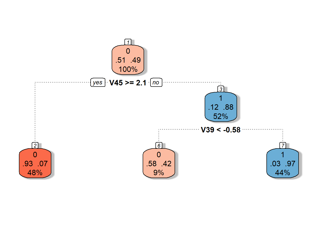
Figure 5.36: Graphical representation of the unpruned decision tree constructed on basis coefficients. Blue shades represent nodes belonging to classification class 1, and red shades represent class 0.
We can also plot the final pruned decision tree.
Code
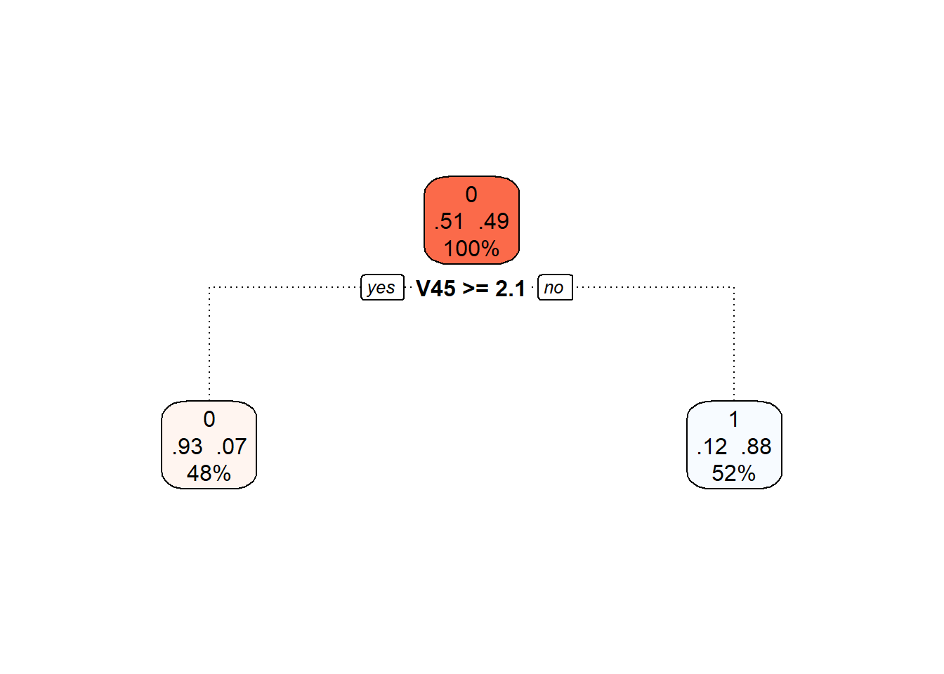
Figure 5.37: Final pruned decision tree.
Finally, we will again add the training and test error rates to the summary table.
5.2.3.6 Random Forests
The classifier constructed using the random forests method consists of building several individual decision trees, which are then combined to create a common classifier (via “voting”).
As with decision trees, we have several options regarding which data (finite-dimensional) we will use to construct the model. We will again consider the three approaches discussed above. The datasets with the corresponding variables for all three approaches have already been prepared from the previous section, so we can directly construct the models, calculate the characteristics of the classifiers, and add the results to the summary table.
5.2.3.6.1 Interval Discretization
In the first case, we utilize the evaluation of functions on a given grid of points over the interval \(I = [0, 6]\).
Code
# model construction
clf.RF <- randomForest(Y ~ ., data = grid.data,
                       ntree = 500, # number of trees
                       importance = TRUE,
                       nodesize = 5)

# accuracy on training data
predictions.train <- predict(clf.RF, newdata = grid.data)
presnost.train <- table(Y.train, predictions.train) |>
  prop.table() |> diag() |> sum()

# accuracy on test data
predictions.test <- predict(clf.RF, newdata = grid.data.test)
presnost.test <- table(Y.test, predictions.test) |>
  prop.table() |> diag() |> sum()
The error rate of the random forest on the training data is thus 0.71 %, and on the test data 13.33 %.
5.2.3.6.2 Principal Component Scores
In this case, we will use the scores of the first $p = $ 3 principal components.
Code
# model construction
clf.RF.PCA <- randomForest(Y ~ ., data = data.PCA.train,
                           ntree = 500, # number of trees
                           importance = TRUE,
                           nodesize = 5)

# accuracy on training data
predictions.train <- predict(clf.RF.PCA, newdata = data.PCA.train)
presnost.train <- table(Y.train, predictions.train) |>
  prop.table() |> diag() |> sum()

# accuracy on test data
predictions.test <- predict(clf.RF.PCA, newdata = data.PCA.test)
presnost.test <- table(Y.test, predictions.test) |>
  prop.table() |> diag() |> sum()
The error rate on the training data is thus 2.86 %, and on the test data 20 %.
5.2.3.6.3 Basis Coefficients
Finally, we will use the representation of functions through the B-spline basis.
Code
# model construction
clf.RF.Bbasis <- randomForest(Y ~ ., data = data.Bbasis.train,
                              ntree = 500, # number of trees
                              importance = TRUE,
                              nodesize = 5)

# accuracy on training data
predictions.train <- predict(clf.RF.Bbasis, newdata = data.Bbasis.train)
presnost.train <- table(Y.train, predictions.train) |>
  prop.table() |> diag() |> sum()

# accuracy on test data
predictions.test <- predict(clf.RF.Bbasis, newdata = data.Bbasis.test)
presnost.test <- table(Y.test, predictions.test) |>
  prop.table() |> diag() |> sum()
The error rate of this classifier on the training data is 0.71 %, and on the test data 10 %.
5.2.3.7 Support Vector Machines
Now let’s look at classifying our simulated curves using the Support Vector Machines (SVM) method. The advantage of this classification method is its computational efficiency, as it defines the boundary curve between classes using only a few (often very few) observations.
In the case of functional data, we have several options for applying the SVM method. The simplest variant is to use this classification method directly on the discretized function (section 5.2.3.7.2). Another option is to utilize the principal component scores to classify curves based on their representation 5.2.3.7.3. A straightforward variant is to use the representation of curves through the B-spline basis and classify curves based on the coefficients of their representation in this basis (section 5.2.3.7.4).
A more complex consideration can lead us to several additional options that leverage the functional nature of the data. We can utilize projections of functions onto a subspace generated, for example, by B-spline functions (section 5.2.3.7.5). The final method we will use for classifying functional data involves combining projection onto a certain subspace generated by functions (Reproducing Kernel Hilbert Space, RKHS) and classifying the corresponding representation. This method utilizes not only the classical SVM but also SVM for regression, as discussed in section RKHS + SVM 5.2.3.7.6.
5.2.3.7.1 SVM for Functional Data
In the fda.usc library, we will use the function classif.svm() to apply the SVM method directly to functional data. First, we will create suitable objects for constructing the classifier.
Code
# set norm equal to one
norms <- c()
for (i in 1:dim(XXder$coefs)[2]) {
  norms <- c(norms, as.numeric(1 / norm.fd(XXder[i])))
}
XXfd_norm <- XXder
XXfd_norm$coefs <- XXfd_norm$coefs * matrix(norms,
                                            ncol = dim(XXder$coefs)[2],
                                            nrow = dim(XXder$coefs)[1],
                                            byrow = TRUE)

# split into test and training sets
X.train_norm <- subset(XXfd_norm, split == TRUE)
X.test_norm <- subset(XXfd_norm, split == FALSE)

Y.train_norm <- subset(Y, split == TRUE)
Y.test_norm <- subset(Y, split == FALSE)

grid.data <- eval.fd(fdobj = X.train_norm, evalarg = t.seq)
grid.data <- as.data.frame(t(grid.data))
grid.data$Y <- Y.train_norm |> factor()

grid.data.test <- eval.fd(fdobj = X.test_norm, evalarg = t.seq)
grid.data.test <- as.data.frame(t(grid.data.test))
grid.data.test$Y <- Y.test_norm |> factor()
Code
# create suitable objects
x.train <- fdata(X.train_norm)
y.train <- as.factor(Y.train_norm)
# points at which the functions are evaluated
tt <- x.train[["argvals"]]
dataf <- as.data.frame(y.train)
colnames(dataf) <- "Y"
# B-spline basis
# basis1 <- X.train_norm$basis
nbasis.x <- 50
basis1 <- create.bspline.basis(rangeval = rangeval,
norder = norder,
nbasis = nbasis.x)Code
# formula
f <- Y ~ x
# basis for x
basis.x <- list("x" = basis1)
# input data for the model
ldata <- list("df" = dataf, "x" = x.train)
# SVM model
model.svm.f <- classif.svm(formula = f,
data = ldata,
basis.x = basis.x,
kernel = 'linear', cost = 1e2)
# accuracy on training data
newdat <- list("x" = x.train)
predictions.train <- predict(model.svm.f, newdat, type = 'class')
presnost.train <- mean(factor(Y.train_norm) == predictions.train)
# accuracy on test data
newdat <- list("x" = fdata(X.test_norm))
predictions.test <- predict(model.svm.f, newdat, type = 'class')
presnost.test <- mean(factor(Y.test_norm) == predictions.test)We calculated the training error (which is 4.29 %) and the test error (which is 8.33 %).
Now let’s attempt, unlike the procedure in the previous chapters, to estimate the hyperparameters of the classifiers from the data using 10-fold cross-validation. Since each kernel has different hyperparameters in its definition, we will approach each kernel function separately. However, the hyperparameter \(C\) appears in all kernel functions, acknowledging that its optimal value may differ between kernels.
For all three kernels, we will explore the values of the hyperparameter \(C\) in the range \([10^{-2}, 10^{5}]\), while for the polynomial kernel, we will consider the value of the hyperparameter \(p\) to be 3, as other integer values do not yield nearly as good results. Conversely, for the radial kernel, we will again use \(r k_cv\)-fold CV to choose the optimal value of the hyperparameter \(\gamma\), considering values in the range \([10^{-5}, 10^{-2}]\). We will set coef0 to 1.
Code
set.seed(42)
k_cv <- 10 # k-fold CV
# We split the training data into k parts
folds <- createMultiFolds(1:sum(split), k = k_cv, time = 1)
# Which values of gamma do we want to consider
gamma.cv <- 10^seq(-5, -2, length = 4)
C.cv <- 10^seq(-2, 5, length = 8)
p.cv <- 3
coef0 <- 1
# A list with three components... an array for each kernel -> linear, poly, radial
# An empty matrix where we will place individual results
# The columns will contain the accuracy values for each
# The rows will correspond to the values for a given gamma and the layers correspond to folds
CV.results <- list(
SVM.l = array(NA, dim = c(length(C.cv), k_cv)),
SVM.p = array(NA, dim = c(length(C.cv), length(p.cv), k_cv)),
SVM.r = array(NA, dim = c(length(C.cv), length(gamma.cv), k_cv))
)
# First, we go through the values of C
for (cost in C.cv) {
# We go through the individual folds
for (index_cv in 1:k_cv) {
# Definition of the test and training parts for CV
fold <- folds[[index_cv]]
cv_sample <- 1:dim(X.train_norm$coefs)[2] %in% fold
x.train.cv <- fdata(subset(X.train_norm, cv_sample))
x.test.cv <- fdata(subset(X.train_norm, !cv_sample))
y.train.cv <- as.factor(subset(Y.train_norm, cv_sample))
y.test.cv <- as.factor(subset(Y.train_norm, !cv_sample))
# Points at which the functions are evaluated
tt <- x.train.cv[["argvals"]]
dataf <- as.data.frame(y.train.cv)
colnames(dataf) <- "Y"
# B-spline basis
# basis1 <- X.train_norm$basis
# Formula
f <- Y ~ x
# Basis for x
basis.x <- list("x" = basis1)
# Input data for the model
ldata <- list("df" = dataf, "x" = x.train.cv)
## LINEAR KERNEL
# SVM model
clf.svm.f_l <- classif.svm(formula = f,
data = ldata,
basis.x = basis.x,
kernel = 'linear',
cost = cost,
type = 'C-classification',
scale = TRUE)
# Accuracy on the test data
newdat <- list("x" = x.test.cv)
predictions.test <- predict(clf.svm.f_l, newdat, type = 'class')
accuracy.test.l <- mean(y.test.cv == predictions.test)
# We insert the accuracies into positions for the given C and fold
CV.results$SVM.l[(1:length(C.cv))[C.cv == cost],
index_cv] <- accuracy.test.l
## POLYNOMIAL KERNEL
for (p in p.cv) {
# Model construction
clf.svm.f_p <- classif.svm(formula = f,
data = ldata,
basis.x = basis.x,
kernel = 'polynomial',
cost = cost,
coef0 = coef0,
degree = p,
type = 'C-classification',
scale = TRUE)
# Accuracy on the test data
newdat <- list("x" = x.test.cv)
predictions.test <- predict(clf.svm.f_p, newdat, type = 'class')
accuracy.test.p <- mean(y.test.cv == predictions.test)
# We insert the accuracies into positions for the given C, p, and fold
CV.results$SVM.p[(1:length(C.cv))[C.cv == cost],
(1:length(p.cv))[p.cv == p],
index_cv] <- accuracy.test.p
}
## RADIAL KERNEL
for (gam.cv in gamma.cv) {
# Model construction
clf.svm.f_r <- classif.svm(formula = f,
data = ldata,
basis.x = basis.x,
kernel = 'radial',
cost = cost,
gamma = gam.cv,
type = 'C-classification',
scale = TRUE)
# Accuracy on the test data
newdat <- list("x" = x.test.cv)
predictions.test <- predict(clf.svm.f_r, newdat, type = 'class')
accuracy.test.r <- mean(y.test.cv == predictions.test)
# We insert the accuracies into positions for the given C, gamma, and fold
CV.results$SVM.r[(1:length(C.cv))[C.cv == cost],
(1:length(gamma.cv))[gamma.cv == gam.cv],
index_cv] <- accuracy.test.r
}
}
}Now we will average the results of 10-fold CV so that we have one estimate of validation error for one value of the hyperparameter (or one combination of values). At the same time, we will determine the optimal values of the individual hyperparameters.
Code
# We calculate the average accuracies for individual C across folds
## Linear kernel
CV.results$SVM.l <- apply(CV.results$SVM.l, 1, mean)
## Polynomial kernel
CV.results$SVM.p <- apply(CV.results$SVM.p, c(1, 2), mean)
## Radial kernel
CV.results$SVM.r <- apply(CV.results$SVM.r, c(1, 2), mean)
C.opt <- c(which.max(CV.results$SVM.l),
which.max(CV.results$SVM.p) %% length(C.cv),
which.max(CV.results$SVM.r) %% length(C.cv))
C.opt[C.opt == 0] <- length(C.cv)
C.opt <- C.cv[C.opt]
gamma.opt <- which.max(t(CV.results$SVM.r)) %% length(gamma.cv)
gamma.opt[gamma.opt == 0] <- length(gamma.cv)
gamma.opt <- gamma.cv[gamma.opt]
p.opt <- which.max(t(CV.results$SVM.p)) %% length(p.cv)
p.opt[p.opt == 0] <- length(p.cv)
p.opt <- p.cv[p.opt]
accuracy.opt.cv <- c(max(CV.results$SVM.l),
max(CV.results$SVM.p),
max(CV.results$SVM.r))Let’s take a look at how the optimal values turned out. For linear kernel, we have the optimal value \(C\) equal to 0.1, for polynomial kernel \(C\) is equal to 1, and for radial kernel, we have two optimal values, for \(C\) the optimal value is 10^{4} and for \(\gamma\) it is 10^{-4}. The validation error rates are 0.1046566 for linear, 0.1266346 for polynomial, and 0.1117995 for radial kernel.
Finally, we can construct the final classifiers on the entire training data with the hyperparameter values determined using 10-fold CV. We will also determine the errors on the test and training data.
Code
# Create suitable objects
x.train <- fdata(X.train_norm)
y.train <- as.factor(Y.train_norm)
# Points at which the functions are evaluated
tt <- x.train[["argvals"]]
dataf <- as.data.frame(y.train)
colnames(dataf) <- "Y"
# B-spline basis
# basis1 <- X.train_norm$basis
# Formula
f <- Y ~ x
# Basis for x
basis.x <- list("x" = basis1)
# Input data for the model
ldata <- list("df" = dataf, "x" = x.train)Code
model.svm.f_l <- classif.svm(formula = f,
data = ldata,
basis.x = basis.x,
kernel = 'linear',
type = 'C-classification',
scale = TRUE,
cost = C.opt[1])
model.svm.f_p <- classif.svm(formula = f,
data = ldata,
basis.x = basis.x,
kernel = 'polynomial',
type = 'C-classification',
scale = TRUE,
degree = p.opt,
coef0 = coef0,
cost = C.opt[2])
model.svm.f_r <- classif.svm(formula = f,
data = ldata,
basis.x = basis.x,
kernel = 'radial',
type = 'C-classification',
scale = TRUE,
gamma = gamma.opt,
cost = C.opt[3])
# Accuracy on training data
newdat <- list("x" = x.train)
predictions.train.l <- predict(model.svm.f_l, newdat, type = 'class')
accuracy.train.l <- mean(factor(Y.train_norm) == predictions.train.l)

predictions.train.p <- predict(model.svm.f_p, newdat, type = 'class')
accuracy.train.p <- mean(factor(Y.train_norm) == predictions.train.p)

predictions.train.r <- predict(model.svm.f_r, newdat, type = 'class')
accuracy.train.r <- mean(factor(Y.train_norm) == predictions.train.r)

# Accuracy on test data
newdat <- list("x" = fdata(X.test_norm))
predictions.test.l <- predict(model.svm.f_l, newdat, type = 'class')
accuracy.test.l <- mean(factor(Y.test_norm) == predictions.test.l)

predictions.test.p <- predict(model.svm.f_p, newdat, type = 'class')
accuracy.test.p <- mean(factor(Y.test_norm) == predictions.test.p)

predictions.test.r <- predict(model.svm.f_r, newdat, type = 'class')
accuracy.test.r <- mean(factor(Y.test_norm) == predictions.test.r)
The error rate of the SVM method on the training data is thus 7.8571 % for the linear kernel, 7.1429 % for the polynomial kernel, and 5.7143 % for the Gaussian kernel. On the test data, the error rate of the method is 8.3333 % for the linear kernel, 10 % for the polynomial kernel, and 8.3333 % for the radial kernel.
5.2.3.7.2 Interval Discretization
Let’s continue by applying the Support Vector Machines method directly to the discretized data (evaluation of the function on a grid of points over the interval \(I = [0, 6]\)), considering all three aforementioned kernel functions.
Now, let’s attempt to estimate the hyperparameters of the classifiers from the data using 10-fold cross-validation. Since each kernel has different hyperparameters in its definition, we will approach each kernel function separately. However, the hyperparameter \(C\) appears in all kernel functions, and we allow its optimal value to differ among kernels.
For all three kernels, we will go through the values of the hyperparameter \(C\) in the interval \([10^{-3}, 10^{4}]\), while for the polynomial kernel we will fix the hyperparameter \(p\) at a value of 3, since other integer values do not yield nearly as good results. On the other hand, for the radial kernel, we will use 10-fold CV to choose the optimal value of the hyperparameter \(\gamma\), considering values in the interval \([10^{-5}, 10^{-1}]\). We will set coef0 to 1.
Code
set.seed(42)
k_cv <- 10 # k-fold CV
# Split training data into k parts
folds <- createMultiFolds(1:sum(split), k = k_cv, time = 1)
# Values of gamma to consider
gamma.cv <- 10^seq(-5, -1, length = 5)
C.cv <- 10^seq(-2, 3, length = 6)
p.cv <- 3
coef0 <- 1
# List with three components ... arrays for individual kernels -> linear, poly, radial
# Empty matrices to store the results
# Columns will contain accuracy values for given C
# Rows will contain values for given gamma, and layers correspond to folds
CV.results <- list(
SVM.l = array(NA, dim = c(length(C.cv), k_cv)),
SVM.p = array(NA, dim = c(length(C.cv), length(p.cv), k_cv)),
SVM.r = array(NA, dim = c(length(C.cv), length(gamma.cv), k_cv))
)
# First, we go through the values of C
for (C in C.cv) {
# Go through individual folds
for (index_cv in 1:k_cv) {
# Definition of test and training parts for CV
fold <- folds[[index_cv]]
cv_sample <- 1:dim(grid.data)[1] %in% fold
data.grid.train.cv <- as.data.frame(grid.data[cv_sample, ])
data.grid.test.cv <- as.data.frame(grid.data[!cv_sample, ])
## LINEAR KERNEL
# Model construction
clf.SVM.l <- svm(Y ~ ., data = data.grid.train.cv,
type = 'C-classification',
scale = TRUE,
cost = C,
kernel = 'linear')
# Accuracy on validation data
predictions.test.l <- predict(clf.SVM.l, newdata = data.grid.test.cv)
accuracy.test.l <- table(data.grid.test.cv$Y, predictions.test.l) |>
prop.table() |> diag() |> sum()
# Store accuracy for given C and fold
CV.results$SVM.l[(1:length(C.cv))[C.cv == C],
index_cv] <- accuracy.test.l
## POLYNOMIAL KERNEL
for (p in p.cv) {
# Model construction
clf.SVM.p <- svm(Y ~ ., data = data.grid.train.cv,
type = 'C-classification',
scale = TRUE,
cost = C,
coef0 = coef0,
degree = p,
kernel = 'polynomial')
# Accuracy on validation data
predictions.test.p <- predict(clf.SVM.p, newdata = data.grid.test.cv)
accuracy.test.p <- table(data.grid.test.cv$Y, predictions.test.p) |>
prop.table() |> diag() |> sum()
# Store accuracy for given C, p, and fold
CV.results$SVM.p[(1:length(C.cv))[C.cv == C],
(1:length(p.cv))[p.cv == p],
index_cv] <- accuracy.test.p
}
## RADIAL KERNEL
for (gamma in gamma.cv) {
# Model construction
clf.SVM.r <- svm(Y ~ ., data = data.grid.train.cv,
type = 'C-classification',
scale = TRUE,
cost = C,
gamma = gamma,
kernel = 'radial')
# Accuracy on validation data
predictions.test.r <- predict(clf.SVM.r, newdata = data.grid.test.cv)
accuracy.test.r <- table(data.grid.test.cv$Y, predictions.test.r) |>
prop.table() |> diag() |> sum()
# Store accuracy for given C, gamma, and fold
CV.results$SVM.r[(1:length(C.cv))[C.cv == C],
(1:length(gamma.cv))[gamma.cv == gamma],
index_cv] <- accuracy.test.r
}
}
}Now, let’s average the results of the 10-fold CV so that for each value of the hyperparameter (or one combination of values), we have one estimate of the validation error. In this process, we will also determine the optimal values for the individual hyperparameters.
Code
# Calculate average accuracies for each C across folds
## Linear kernel
CV.results$SVM.l <- apply(CV.results$SVM.l, 1, mean)
## Polynomial kernel
CV.results$SVM.p <- apply(CV.results$SVM.p, c(1, 2), mean)
## Radial kernel
CV.results$SVM.r <- apply(CV.results$SVM.r, c(1, 2), mean)
C.opt <- c(which.max(CV.results$SVM.l),
which.max(CV.results$SVM.p) %% length(C.cv),
which.max(CV.results$SVM.r) %% length(C.cv))
C.opt[C.opt == 0] <- length(C.cv)
C.opt <- C.cv[C.opt]
gamma.opt <- which.max(t(CV.results$SVM.r)) %% length(gamma.cv)
gamma.opt[gamma.opt == 0] <- length(gamma.cv)
gamma.opt <- gamma.cv[gamma.opt]
p.opt <- which.max(t(CV.results$SVM.p)) %% length(p.cv)
p.opt[p.opt == 0] <- length(p.cv)
p.opt <- p.cv[p.opt]
accuracy.opt.cv <- c(max(CV.results$SVM.l),
max(CV.results$SVM.p),
max(CV.results$SVM.r))Let’s look at how the optimal values turned out. For the linear kernel, the optimal value of \(C\) is 0.01, for the polynomial kernel \(C\) is 0.1, and for the radial kernel, we have two optimal values: for \(C\), the optimal value is 1000, and for \(\gamma\), it is 10^{-4}. The validation errors are 0.1067399 for linear, 0.1373031 for polynomial, and 0.0991804 for radial kernels.
Finally, we can construct the final classifiers on the entire training data with the hyperparameter values determined by 10-fold CV. We will also determine the errors on both test and training datasets.
Code
# Model construction
clf.SVM.l <- svm(Y ~ ., data = grid.data,
type = 'C-classification',
scale = TRUE,
cost = C.opt[1],
kernel = 'linear')
clf.SVM.p <- svm(Y ~ ., data = grid.data,
type = 'C-classification',
scale = TRUE,
cost = C.opt[2],
degree = p.opt,
coef0 = coef0,
kernel = 'polynomial')
clf.SVM.r <- svm(Y ~ ., data = grid.data,
type = 'C-classification',
scale = TRUE,
cost = C.opt[3],
gamma = gamma.opt,
kernel = 'radial')
# Accuracy on training data
predictions.train.l <- predict(clf.SVM.l, newdata = grid.data)
accuracy.train.l <- table(Y.train, predictions.train.l) |>
prop.table() |> diag() |> sum()
predictions.train.p <- predict(clf.SVM.p, newdata = grid.data)
accuracy.train.p <- table(Y.train, predictions.train.p) |>
prop.table() |> diag() |> sum()
predictions.train.r <- predict(clf.SVM.r, newdata = grid.data)
accuracy.train.r <- table(Y.train, predictions.train.r) |>
prop.table() |> diag() |> sum()
# Accuracy on test data
predictions.test.l <- predict(clf.SVM.l, newdata = grid.data.test)
accuracy.test.l <- table(Y.test, predictions.test.l) |>
prop.table() |> diag() |> sum()
predictions.test.p <- predict(clf.SVM.p, newdata = grid.data.test)
accuracy.test.p <- table(Y.test, predictions.test.p) |>
prop.table() |> diag() |> sum()
predictions.test.r <- predict(clf.SVM.r, newdata = grid.data.test)
accuracy.test.r <- table(Y.test, predictions.test.r) |>
prop.table() |> diag() |> sum()The error rate of the SVM method on the training data is 9.2857 % for the linear kernel, 9.2857 % for the polynomial kernel, and 6.4286 % for the Gaussian kernel. On the test data, the error rate is 10 % for the linear kernel, 10 % for the polynomial kernel, and 10 % for the radial kernel.
5.2.3.7.3 Principal Component Scores
In this case, we will use the scores of the first \(p =\) 3 principal components.
Now, let’s try, unlike the approach in previous chapters, to estimate the classifier hyperparameters from the data using 10-fold cross-validation. Given that each kernel has different hyperparameters in its definition, we will treat each kernel function separately. However, the hyperparameter \(C\) appears in all kernel functions, although we allow that its optimal value may differ between kernels.
For all three kernels, we will test values of the hyperparameter \(C\) in the interval \([10^{-3}, 10^{3}]\). For the polynomial kernel, we fix the hyperparameter \(p\) at the value of 3, as for other integer values, the method does not give nearly as good results. In contrast, for the radial kernel, we will use 10-fold CV to choose the optimal value of the hyperparameter \(\gamma\), considering values in the interval \([10^{-5}, 10^{-2}]\). We set coef0 \(= 1\).
Code
set.seed(42)
# gamma values to consider
gamma.cv <- 10^seq(-4, -1, length = 4)
C.cv <- 10^seq(-3, 3, length = 7)
p.cv <- 3
coef0 <- 1
# list with three components ... array for individual kernels -> linear, poly, radial
# empty matrix to store results
# columns will have accuracy values for a given
# rows will have values for given gamma and layers correspond to folds
CV.results <- list(
SVM.l = array(NA, dim = c(length(C.cv), k_cv)),
SVM.p = array(NA, dim = c(length(C.cv), length(p.cv), k_cv)),
SVM.r = array(NA, dim = c(length(C.cv), length(gamma.cv), k_cv))
)
# first, go through C values
for (C in C.cv) {
# iterate over each fold
for (index_cv in 1:k_cv) {
# define test and training parts for CV
fold <- folds[[index_cv]]
cv_sample <- 1:dim(data.PCA.train)[1] %in% fold
data.PCA.train.cv <- as.data.frame(data.PCA.train[cv_sample, ])
data.PCA.test.cv <- as.data.frame(data.PCA.train[!cv_sample, ])
## LINEAR KERNEL
# build model
clf.SVM.l <- svm(Y ~ ., data = data.PCA.train.cv,
type = 'C-classification',
scale = TRUE,
cost = C,
kernel = 'linear')
# accuracy on validation data
predictions.test.l <- predict(clf.SVM.l, newdata = data.PCA.test.cv)
presnost.test.l <- table(data.PCA.test.cv$Y, predictions.test.l) |>
prop.table() |> diag() |> sum()
# store accuracies for given C and fold
CV.results$SVM.l[(1:length(C.cv))[C.cv == C],
index_cv] <- presnost.test.l
## POLYNOMIAL KERNEL
for (p in p.cv) {
# build model
clf.SVM.p <- svm(Y ~ ., data = data.PCA.train.cv,
type = 'C-classification',
scale = TRUE,
cost = C,
coef0 = coef0,
degree = p,
kernel = 'polynomial')
# accuracy on validation data
predictions.test.p <- predict(clf.SVM.p, newdata = data.PCA.test.cv)
presnost.test.p <- table(data.PCA.test.cv$Y, predictions.test.p) |>
prop.table() |> diag() |> sum()
# store accuracies for given C, p, and fold
CV.results$SVM.p[(1:length(C.cv))[C.cv == C],
(1:length(p.cv))[p.cv == p],
index_cv] <- presnost.test.p
}
## RADIAL KERNEL
for (gamma in gamma.cv) {
# build model
clf.SVM.r <- svm(Y ~ ., data = data.PCA.train.cv,
type = 'C-classification',
scale = TRUE,
cost = C,
gamma = gamma,
kernel = 'radial')
# accuracy on validation data
predictions.test.r <- predict(clf.SVM.r, newdata = data.PCA.test.cv)
presnost.test.r <- table(data.PCA.test.cv$Y, predictions.test.r) |>
prop.table() |> diag() |> sum()
# store accuracies for given C, gamma, and fold
CV.results$SVM.r[(1:length(C.cv))[C.cv == C],
(1:length(gamma.cv))[gamma.cv == gamma],
index_cv] <- presnost.test.r
}
}
}Now we average the results of the 10-fold CV to obtain a single estimate of validation error for each hyperparameter value (or combination of values). We also determine the optimal values of each hyperparameter.
Code
# calculate average accuracies for individual C over folds
## Linear kernel
CV.results$SVM.l <- apply(CV.results$SVM.l, 1, mean)
## Polynomial kernel
CV.results$SVM.p <- apply(CV.results$SVM.p, c(1, 2), mean)
## Radial kernel
CV.results$SVM.r <- apply(CV.results$SVM.r, c(1, 2), mean)
C.opt <- c(which.max(CV.results$SVM.l),
which.max(CV.results$SVM.p) %% length(C.cv),
which.max(CV.results$SVM.r) %% length(C.cv))
C.opt[C.opt == 0] <- length(C.cv)
C.opt <- C.cv[C.opt]
gamma.opt <- which.max(t(CV.results$SVM.r)) %% length(gamma.cv)
gamma.opt[gamma.opt == 0] <- length(gamma.cv)
gamma.opt <- gamma.cv[gamma.opt]
p.opt <- which.max(t(CV.results$SVM.p)) %% length(p.cv)
p.opt[p.opt == 0] <- length(p.cv)
p.opt <- p.cv[p.opt]
presnost.opt.cv <- c(max(CV.results$SVM.l),
max(CV.results$SVM.p),
max(CV.results$SVM.r))Let’s look at how the optimal values turned out. For the linear kernel, the optimal value of \(C\) is 0.01, for the polynomial kernel \(C\) is 0.01, and for the radial kernel, there are two optimal values: \(C\) is 100 and \(\gamma\) is 0.01. The validation errors are 0.128837 for linear, 0.1227198 for polynomial, and 0.1216941 for the radial kernel.
Finally, we can construct the final classifiers on the entire training dataset with hyperparameter values determined using 10-fold CV. We also calculate errors on the test and training datasets.
Code
# build model
clf.SVM.l.PCA <- svm(Y ~ ., data = data.PCA.train,
type = 'C-classification',
scale = TRUE,
cost = C.opt[1],
kernel = 'linear')
clf.SVM.p.PCA <- svm(Y ~ ., data = data.PCA.train,
type = 'C-classification',
scale = TRUE,
cost = C.opt[2],
degree = p.opt,
coef0 = coef0,
kernel = 'polynomial')
clf.SVM.r.PCA <- svm(Y ~ ., data = data.PCA.train,
type = 'C-classification',
scale = TRUE,
cost = C.opt[3],
gamma = gamma.opt,
kernel = 'radial')
# accuracy on training data
predictions.train.l <- predict(clf.SVM.l.PCA, newdata = data.PCA.train)
presnost.train.l <- table(data.PCA.train$Y, predictions.train.l) |>
prop.table() |> diag() |> sum()
predictions.train.p <- predict(clf.SVM.p.PCA, newdata = data.PCA.train)
presnost.train.p <- table(data.PCA.train$Y, predictions.train.p) |>
prop.table() |> diag() |> sum()
predictions.train.r <- predict(clf.SVM.r.PCA, newdata = data.PCA.train)
presnost.train.r <- table(data.PCA.train$Y, predictions.train.r) |>
prop.table() |> diag() |> sum()
# accuracy on test data
predictions.test.l <- predict(clf.SVM.l.PCA, newdata = data.PCA.test)
presnost.test.l <- table(data.PCA.test$Y, predictions.test.l) |>
prop.table() |> diag() |> sum()
predictions.test.p <- predict(clf.SVM.p.PCA, newdata = data.PCA.test)
presnost.test.p <- table(data.PCA.test$Y, predictions.test.p) |>
prop.table() |> diag() |> sum()
predictions.test.r <- predict(clf.SVM.r.PCA, newdata = data.PCA.test)
presnost.test.r <- table(data.PCA.test$Y, predictions.test.r) |>
prop.table() |> diag() |> sum()The training accuracies are 0.8642857 for linear, 0.8714286 for polynomial, and 0.8642857 for radial kernels, and the test accuracies are 0.8166667 for linear, 0.8166667 for polynomial, and 0.8333333 for radial.
To visualize the method, we can plot the decision boundary on a graph of the scores for the first two principal components. We compute this boundary on a dense grid of points and display it using the geom_contour() function, just as in previous cases where we also plotted the classification boundary.
Code
nd <- rbind(nd, nd, nd) |> mutate(
prd = c(as.numeric(predict(clf.SVM.l.PCA, newdata = nd, type = 'response')),
as.numeric(predict(clf.SVM.p.PCA, newdata = nd, type = 'response')),
as.numeric(predict(clf.SVM.r.PCA, newdata = nd, type = 'response'))),
kernel = rep(c('linear', 'polynomial', 'radial'),
each = length(as.numeric(predict(clf.SVM.l.PCA,
newdata = nd,
type = 'response')))) |>
as.factor())
data.PCA.train |> ggplot(aes(x = V1, y = V2, colour = Y)) +
geom_point(size = 1.5) +
labs(x = paste('1st Principal Component (Explained Variance',
round(100 * data.PCA$varprop[1], 2), '%)'),
y = paste('2nd Principal Component (',
round(100 * data.PCA$varprop[2], 2), '%)'),
colour = 'Fat Content',
linetype = 'Kernel') +
scale_colour_discrete(labels = c("low", "high")) +
theme_bw() +
geom_contour(data = nd, aes(x = V1, y = V2, z = prd, linetype = kernel),
colour = 'black') 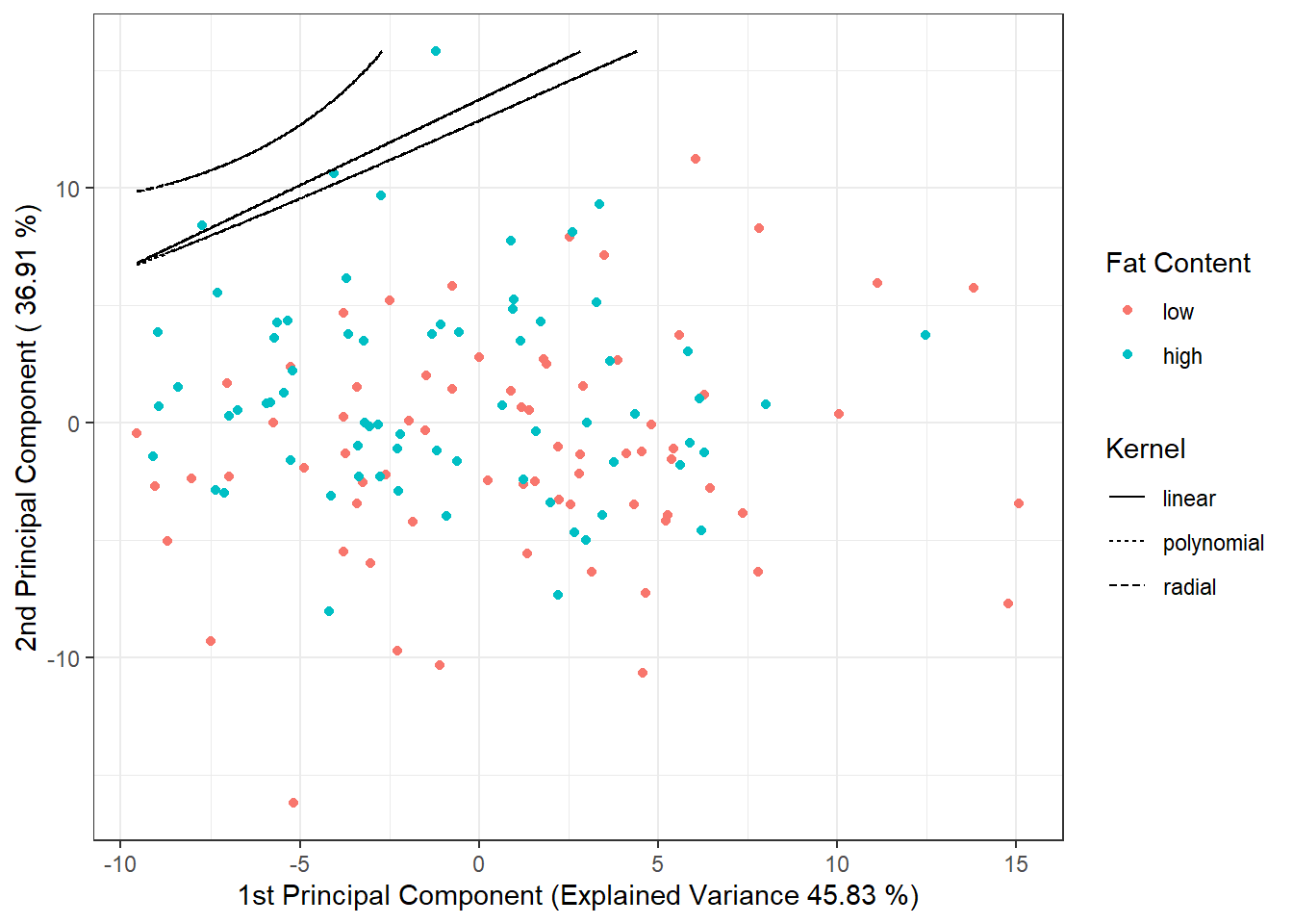
Figure 5.38: Scores of the first two principal components, color-coded by classification group. The decision boundary (either a line or curves in the plane of the first two principal components) between classes is displayed in black, created using the SVM method.
5.2.3.7.4 B-spline Coefficients
Finally, we use a B-spline basis to express the functions. For all three kernels, we examine the values of hyperparameter \(C\) in the interval \([10^{-1}, 10^{3}]\). For the polynomial kernel, we fix the hyperparameter \(p\) at 3, as other integer values do not yield nearly as good results. On the other hand, for the radial kernel, we again use 10-fold CV to select the optimal value of hyperparameter \(\gamma\), considering values in the interval \([10^{-5}, 10^{-1}]\). We set coef0 \(= 1\).
Code
set.seed(42)
# gamma values to consider
gamma.cv <- 10^seq(-5, -1, length = 5)
C.cv <- 10^seq(-2, 2, length = 5)
p.cv <- 3
coef0 <- 1
# list with three components...array for each kernel -> linear, poly, radial
# empty matrix to store individual results
# columns hold accuracy values for given
# rows represent values for given gamma, and layers correspond to folds
CV.results <- list(
SVM.l = array(NA, dim = c(length(C.cv), k_cv)),
SVM.p = array(NA, dim = c(length(C.cv), length(p.cv), k_cv)),
SVM.r = array(NA, dim = c(length(C.cv), length(gamma.cv), k_cv))
)
# first iterate through values of C
for (C in C.cv) {
# iterate over individual folds
for (index_cv in 1:k_cv) {
# define test and training parts for CV
fold <- folds[[index_cv]]
cv_sample <- 1:dim(grid.data)[1] %in% fold
data.Bbasis.train.cv <- as.data.frame(data.Bbasis.train[cv_sample, ])
data.Bbasis.test.cv <- as.data.frame(data.Bbasis.train[!cv_sample, ])
## LINEAR KERNEL
# model creation
clf.SVM.l <- svm(Y ~ ., data = data.Bbasis.train.cv,
type = 'C-classification',
scale = TRUE,
cost = C,
kernel = 'linear')
# accuracy on validation data
predictions.test.l <- predict(clf.SVM.l, newdata = data.Bbasis.test.cv)
presnost.test.l <- table(data.Bbasis.test.cv$Y, predictions.test.l) |>
prop.table() |> diag() |> sum()
# insert accuracies in positions for given C and fold
CV.results$SVM.l[(1:length(C.cv))[C.cv == C],
index_cv] <- presnost.test.l
## POLYNOMIAL KERNEL
for (p in p.cv) {
# model creation
clf.SVM.p <- svm(Y ~ ., data = data.Bbasis.train.cv,
type = 'C-classification',
scale = TRUE,
cost = C,
coef0 = coef0,
degree = p,
kernel = 'polynomial')
# accuracy on validation data
predictions.test.p <- predict(clf.SVM.p,
newdata = data.Bbasis.test.cv)
presnost.test.p <- table(data.Bbasis.test.cv$Y, predictions.test.p) |>
prop.table() |> diag() |> sum()
# insert accuracies in positions for given C, p, and fold
CV.results$SVM.p[(1:length(C.cv))[C.cv == C],
(1:length(p.cv))[p.cv == p],
index_cv] <- presnost.test.p
}
## RADIAL KERNEL
for (gamma in gamma.cv) {
# model creation
clf.SVM.r <- svm(Y ~ ., data = data.Bbasis.train.cv,
type = 'C-classification',
scale = TRUE,
cost = C,
gamma = gamma,
kernel = 'radial')
# accuracy on validation data
predictions.test.r <- predict(clf.SVM.r,
newdata = data.Bbasis.test.cv)
presnost.test.r <- table(data.Bbasis.test.cv$Y, predictions.test.r) |>
prop.table() |> diag() |> sum()
# insert accuracies in positions for given C, gamma, and fold
CV.results$SVM.r[(1:length(C.cv))[C.cv == C],
(1:length(gamma.cv))[gamma.cv == gamma],
index_cv] <- presnost.test.r
}
}
}Now we average the results from 10-fold CV so that we have a single estimate of validation error for each hyperparameter value (or combination of values). We also determine the optimal values of each hyperparameter.
Code
# calculate average accuracies for each C across folds
## Linear kernel
CV.results$SVM.l <- apply(CV.results$SVM.l, 1, mean)
## Polynomial kernel
CV.results$SVM.p <- apply(CV.results$SVM.p, c(1, 2), mean)
## Radial kernel
CV.results$SVM.r <- apply(CV.results$SVM.r, c(1, 2), mean)
C.opt <- c(which.max(CV.results$SVM.l),
which.max(CV.results$SVM.p) %% length(C.cv),
which.max(CV.results$SVM.r) %% length(C.cv))
C.opt[C.opt == 0] <- length(C.cv)
C.opt <- C.cv[C.opt]
gamma.opt <- which.max(t(CV.results$SVM.r)) %% length(gamma.cv)
gamma.opt[gamma.opt == 0] <- length(gamma.cv)
gamma.opt <- gamma.cv[gamma.opt]
p.opt <- which.max(t(CV.results$SVM.p)) %% length(p.cv)
p.opt[p.opt == 0] <- length(p.cv)
p.opt <- p.cv[p.opt]
presnost.opt.cv <- c(max(CV.results$SVM.l),
max(CV.results$SVM.p),
max(CV.results$SVM.r))Let’s see how the optimal values turned out. For the linear kernel, the optimal \(C\) value is 0.1, for the polynomial kernel, \(C\) is 0.1, and for the radial kernel, we have two optimal values: \(C\) is 10, and \(\gamma\) is 0.01. The validation error rates are 0.099359 for linear, 0.1208013 for polynomial, and 0.0792399 for radial kernels.
Finally, we can construct the final classifiers on the entire training dataset using the hyperparameter values determined by 10-fold CV. We will also calculate the error rates on both the test and training data.
Code
# Model construction
clf.SVM.l.Bbasis <- svm(Y ~ ., data = data.Bbasis.train,
type = 'C-classification',
scale = TRUE,
cost = C.opt[1],
kernel = 'linear')
clf.SVM.p.Bbasis <- svm(Y ~ ., data = data.Bbasis.train,
type = 'C-classification',
scale = TRUE,
cost = C.opt[2],
degree = p.opt,
coef0 = coef0,
kernel = 'polynomial')
clf.SVM.r.Bbasis <- svm(Y ~ ., data = data.Bbasis.train,
type = 'C-classification',
scale = TRUE,
cost = C.opt[3],
gamma = gamma.opt,
kernel = 'radial')
# Accuracy on training data
predictions.train.l <- predict(clf.SVM.l.Bbasis, newdata = data.Bbasis.train)
presnost.train.l <- table(Y.train, predictions.train.l) |>
prop.table() |> diag() |> sum()
predictions.train.p <- predict(clf.SVM.p.Bbasis, newdata = data.Bbasis.train)
presnost.train.p <- table(Y.train, predictions.train.p) |>
prop.table() |> diag() |> sum()
predictions.train.r <- predict(clf.SVM.r.Bbasis, newdata = data.Bbasis.train)
presnost.train.r <- table(Y.train, predictions.train.r) |>
prop.table() |> diag() |> sum()
# Accuracy on test data
predictions.test.l <- predict(clf.SVM.l.Bbasis, newdata = data.Bbasis.test)
presnost.test.l <- table(Y.test, predictions.test.l) |>
prop.table() |> diag() |> sum()
predictions.test.p <- predict(clf.SVM.p.Bbasis, newdata = data.Bbasis.test)
presnost.test.p <- table(Y.test, predictions.test.p) |>
prop.table() |> diag() |> sum()
predictions.test.r <- predict(clf.SVM.r.Bbasis, newdata = data.Bbasis.test)
presnost.test.r <- table(Y.test, predictions.test.r) |>
prop.table() |> diag() |> sum()The error rate of the SVM method applied to the basis coefficients on the training data is 5.71% for the linear kernel, 9.29% for the polynomial kernel, and 1.43% for the Gaussian kernel.
On the test data, the error rate is 6.6667% for the linear kernel, 6.6667% for the polynomial kernel, and 8.3333% for the radial kernel.
5.2.3.7.5 Projection onto B-spline Basis
Another option for using the classical SVM method for functional data is to project the original data onto some \(d\)-dimensional subspace of our Hilbert space \(\mathcal{H}\), denoted as \(V_d\). Assume that this subspace \(V_d\) has an orthonormal basis \(\{\Psi_j\}_{j = 1, \dots, d}\). We define the transformation \(P_{V_d}\) as the orthogonal projection onto the subspace \(V_d\), so we can write:
\[ P_{V_d} (x) = \sum_{j = 1}^d \langle x, \Psi_j \rangle \Psi_j. \]
Now we can use the coefficients from the orthogonal projection for classification, that is, we apply the standard SVM to the vectors \(\left( \langle x, \Psi_1 \rangle, \dots, \langle x, \Psi_d \rangle\right)^\top\). By using this transformation, we have defined a new so-called adapted kernel, which consists of the orthogonal projection \(P_{V_d}\) and the kernel function of the standard support vector method. Thus, we have (adapted) kernel \(Q(x_i, x_j) = K(P_{V_d}(x_i), P_{V_d}(x_j))\). This is a dimensionality reduction method, which we can call filtering.
For the projection itself, we will use the project.basis() function from the fda library in R. Its input will be a matrix of the original discrete (non-smoothed) data, the values at which we measure values in the original data matrix, and the basis object onto which we want to project the data. We will choose projection onto a B-spline basis since the use of a Fourier basis is not suitable for our non-periodic data.
We choose the dimension \(d\) either from some prior expert knowledge or by using cross-validation. In our case, we will determine the optimal dimension of the subspace \(V_d\) using \(k\)-fold cross-validation (we choose \(k \ll n\) due to the computational intensity of the method, often \(k = 5\) or \(k = 10\)). We require B-splines of order 4, for which the relationship for the number of basis functions holds:
\[ n_{basis} = n_{breaks} + n_{order} - 2, \]
where \(n_{breaks}\) is the number of knots and \(n_{order} = 4\). Therefore, the minimum dimension (for \(n_{breaks} = 1\)) is chosen as \(n_{basis} = 3\), and the maximum (for \(n_{breaks} = 51\), corresponding to the number of original discrete data points) is \(n_{basis} = 53\). However, in R, the value of \(n_{basis}\) must be at least \(n_{order} = 4\), and for large values of \(n_{basis}\), we already experience model overfitting; therefore, we choose a maximum \(n_{basis}\) of a smaller number, say 43.
Code
k_cv <- 10 # k-fold CV

# Values for B-spline basis
rangeval <- range(t)
norder <- 4
n_basis_min <- norder
n_basis_max <- length(t) + norder - 2 - 10

dimensions <- n_basis_min:n_basis_max # all dimensions we want to try

# Split the training data into k parts
folds <- createMultiFolds(1:sum(split), k = k_cv, time = 1)

# List with three components ... matrices for individual kernels -> linear, poly, radial
# An empty matrix where we will insert individual results
# Columns will contain accuracy values for each part of the training set
# Rows will contain values for each dimension value
CV.results <- list(SVM.l = matrix(NA, nrow = length(dimensions), ncol = k_cv),
                   SVM.p = matrix(NA, nrow = length(dimensions), ncol = k_cv),
                   SVM.r = matrix(NA, nrow = length(dimensions), ncol = k_cv))

for (d in dimensions) {
  # Basis object
  bbasis <- create.bspline.basis(rangeval = rangeval,
                                 nbasis = d)

  # Projection of discrete data onto the B-spline basis of dimension d
  Projection <- project.basis(y = grid.data |> select(!contains('Y')) |> as.matrix() |> t(), # matrix of discrete data
                              argvals = t.seq, # vector of arguments
                              basisobj = bbasis) # basis object

  # Splitting into training and test data within CV
  XX.train <- t(Projection) # subset(t(Projection), split == TRUE)

  for (index_cv in 1:k_cv) {
    # Definition of test and training parts for CV
    fold <- folds[[index_cv]]
    cv_sample <- 1:dim(XX.train)[1] %in% fold

    data.projection.train.cv <- as.data.frame(XX.train[cv_sample, ])
    data.projection.train.cv$Y <- factor(Y.train[cv_sample])

    data.projection.test.cv <- as.data.frame(XX.train[!cv_sample, ])
    Y.test.cv <- Y.train[!cv_sample]
    data.projection.test.cv$Y <- factor(Y.test.cv)

    # Building the models
    clf.SVM.l.projection <- svm(Y ~ ., data = data.projection.train.cv,
                            type = 'C-classification',
                            scale = TRUE,
                            kernel = 'linear')

    clf.SVM.p.projection <- svm(Y ~ ., data = data.projection.train.cv,
                            type = 'C-classification',
                            scale = TRUE,
                            coef0 = 1,
                            kernel = 'polynomial')

    clf.SVM.r.projection <- svm(Y ~ ., data = data.projection.train.cv,
                            type = 'C-classification',
                            scale = TRUE,
                            kernel = 'radial')

    # Accuracy on validation data
    ## linear kernel
    predictions.test.l <- predict(clf.SVM.l.projection,
                                  newdata = data.projection.test.cv)
    accuracy.test.l <- table(Y.test.cv, predictions.test.l) |>
      prop.table() |> diag() |> sum()
    ## polynomial kernel
    predictions.test.p <- predict(clf.SVM.p.projection,
                                  newdata = data.projection.test.cv)
    accuracy.test.p <- table(Y.test.cv, predictions.test.p) |>
      prop.table() |> diag() |> sum()
    ## radial kernel
    predictions.test.r <- predict(clf.SVM.r.projection,
                                  newdata = data.projection.test.cv)
    accuracy.test.r <- table(Y.test.cv, predictions.test.r) |>
      prop.table() |> diag() |> sum()

    # Insert accuracies into positions for given d and fold
    CV.results$SVM.l[d - min(dimensions) + 1, index_cv] <- accuracy.test.l
    CV.results$SVM.p[d - min(dimensions) + 1, index_cv] <- accuracy.test.p
    CV.results$SVM.r[d - min(dimensions) + 1, index_cv] <- accuracy.test.r
  }
}

# Compute average accuracies for individual d across folds
for (n_method in 1:length(CV.results)) {
  CV.results[[n_method]] <- apply(CV.results[[n_method]], 1, mean)
}

d.opt <- c(which.max(CV.results$SVM.l) + n_basis_min - 1,
           which.max(CV.results$SVM.p) + n_basis_min - 1,
           which.max(CV.results$SVM.r) + n_basis_min - 1)
presnost.opt.cv <- c(max(CV.results$SVM.l),
                     max(CV.results$SVM.p),
                     max(CV.results$SVM.r))
data.frame(d_opt = d.opt, ERR = 1 - presnost.opt.cv,
           row.names = c('linear', 'poly', 'radial'))
## d_opt ERR
## linear 16 0.10007326
## poly 11 0.11804945
## radial 11 0.09126374We see that the best value for the parameter \(d\) is 16 for the linear kernel, with an error rate calculated using 10-fold CV of 0.1001, 11 for the polynomial kernel with an error rate of 0.118, and 11 for the radial kernel with an error rate of 0.0913.
To clarify, let’s plot the validation error rates as a function of the dimension \(d\).
Code
CV.results <- data.frame(d = dimensions |> rep(3),
                         CV = c(CV.results$SVM.l,
                                CV.results$SVM.p,
                                CV.results$SVM.r),
                         Kernel = rep(c('linear', 'polynomial', 'radial'),
                                      each = length(dimensions)) |> factor())
CV.results |> ggplot(aes(x = d, y = 1 - CV, colour = Kernel)) +
  geom_line(linetype = 'dashed') +
  geom_point(size = 1.5) +
  geom_point(data = data.frame(d.opt,
                               presnost.opt.cv),
             aes(x = d.opt, y = 1 - presnost.opt.cv), colour = 'black', size = 2) +
  theme_bw() +
  labs(x = bquote(paste(d)),
       y = 'Validation error rate') +
  theme(legend.position = "bottom") +
  scale_x_continuous(breaks = dimensions)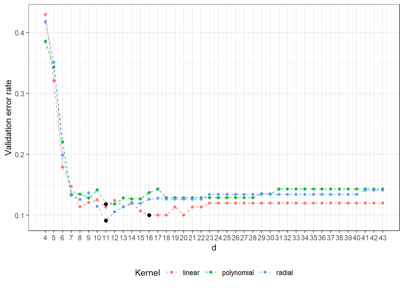
Figure 5.39: Dependency of validation error rate on the dimension of the subspace \(V_d\), separately for all three considered kernels in the SVM method. The optimal values of the dimension \(V_d\) for each kernel function are marked with black points.
Now we can train the individual classifiers on all training data and examine their performance on the test data. For each kernel function, we choose the dimension of the subspace to project onto according to the results of cross-validation.
The variable Projection stores the matrix of coefficients from the orthogonal projection, that is,
\[ \texttt{Projection} = \begin{pmatrix} \langle x_1, \Psi_1 \rangle & \langle x_2, \Psi_1 \rangle & \cdots & \langle x_n, \Psi_1 \rangle\\ \langle x_1, \Psi_2 \rangle & \langle x_2, \Psi_2 \rangle & \cdots & \langle x_n, \Psi_2 \rangle\\ \vdots & \vdots & \ddots & \vdots \\ \langle x_1, \Psi_d \rangle & \langle x_2, \Psi_d \rangle & \dots & \langle x_n, \Psi_d \rangle \end{pmatrix}_{d \times n}. \]
Code
# Prepare a data table to store results
Res <- data.frame(model = c('SVM linear - projection',
                            'SVM poly - projection',
                            'SVM rbf - projection'),
                  Err.train = NA,
                  Err.test = NA)

# Loop through each kernel
for (kernel_number in 1:3) {
  kernel_type <- c('linear', 'polynomial', 'radial')[kernel_number]
  # Base object
  bbasis <- create.bspline.basis(rangeval = rangeval,
                                 nbasis = d.opt[kernel_number])

  # Project discrete data onto B-spline basis
  Projection <- project.basis(y = rbind(
    grid.data |> select(!contains('Y')),
    grid.data.test |> select(!contains('Y'))) |>
      as.matrix() |> t(), # Matrix of discrete data
                              argvals = t.seq, # Vector of arguments
                              basisobj = bbasis) # Basis object

  # Split into training and testing data
  XX.train <- t(Projection)[1:sum(split), ]
  XX.test <- t(Projection)[(sum(split) + 1):length(split), ]

  data.projection.train <- as.data.frame(XX.train)
  data.projection.train$Y <- factor(Y.train)

  data.projection.test <- as.data.frame(XX.test)
  data.projection.test$Y <- factor(Y.test)

  # Construct the model
  clf.SVM.projection <- svm(Y ~ ., data = data.projection.train,
                            type = 'C-classification',
                            scale = TRUE,
                            coef0 = 1,
                            kernel = kernel_type)

  # Accuracy on training data
  predictions.train <- predict(clf.SVM.projection, newdata = data.projection.train)
  presnost.train <- table(Y.train, predictions.train) |>
    prop.table() |> diag() |> sum()

  # Accuracy on testing data
  predictions.test <- predict(clf.SVM.projection, newdata = data.projection.test)
  presnost.test <- table(Y.test, predictions.test) |>
    prop.table() |> diag() |> sum()

  # Store results
  Res[kernel_number, c(2, 3)] <- 1 - c(presnost.train, presnost.test)
}
The error rate of the SVM method applied to the basis coefficients on the training data is therefore 5 % for the linear kernel, 2.86 % for the polynomial kernel, and 5 % for the Gaussian kernel. On the test data, the error rates are 8.33 % for the linear kernel, 11.67 % for the polynomial kernel, and 8.33 % for the radial kernel.
5.2.3.7.6 RKHS + SVM
In this section, we will explore another way to utilize support vector machines (SVM) for classifying functional data. Here, we will again rely on the familiar principle of first expressing functional data as finite-dimensional objects and then applying the traditional SVM method to these objects.
However, this time we will use the SVM method for the representation of functional data itself via a certain finite-dimensional object. As the name suggests, this involves a combination of two concepts: the support vector machine method and a space referred to in English literature as Reproducing Kernel Hilbert Space (RKHS). A key concept in this space is the kernel.
5.2.3.7.6.1 Implementation of the Method in R
From the last part of Theorem 1.3, we can see how to compute the representations of curves in practice. We will work with discretized data after smoothing the curves. First, let’s define a kernel for the RKHS space. We will use the Gaussian kernel with a parameter \(\gamma\). The value of this hyperparameter significantly affects the behaviour and success of the method, so we must pay special attention to its choice (we select it using cross-validation).
5.2.3.7.6.2 Gaussian Kernel
Code
# Remove the last column, which contains the values of Y
data.RKHS <- grid.data[, -dim(grid.data)[2]] |> t()
# Add test data as well
data.RKHS <- cbind(data.RKHS, grid.data.test[, -dim(grid.data.test)[2]] |> t())

# Kernel and kernel matrix ... Gaussian with parameter gamma
Gauss.kernel <- function(x, y, gamma) {
  return(exp(-gamma * norm(c(x - y) |> t(), type = 'F')))
}

Kernel.RKHS <- function(x, gamma) {
  K <- matrix(NA, ncol = length(x), nrow = length(x))
  for(i in 1:nrow(K)) {
    for(j in 1:ncol(K)) {
      K[i, j] <- Gauss.kernel(x = x[i], y = x[j], gamma = gamma)
    }
  }
  return(K)
}
Now let’s compute the matrix \(K_S\) along with its eigenvalues and corresponding eigenvectors.
Code
To compute the coefficients in the representation of the curves, that is, to calculate the vectors \(\hat{\boldsymbol \lambda}_l^* = \left( \hat\lambda_{1l}^*, \dots, \hat\lambda_{\hat dl}^*\right)^\top, l = 1, 2, \dots, n\), we also need the coefficients from SVM. Unlike the classification problem, we are now solving a regression problem, as we are trying to express our observed curves in some basis chosen by the kernel \(K\). Therefore, we will use the Support Vector Regression method, from which we will obtain the coefficients \(\alpha_{il}\).
Code
# Determine coefficients alpha from SVM
alpha.RKHS <- matrix(0, nrow = dim(data.RKHS)[1],
                     ncol = dim(data.RKHS)[2]) # Empty object

# Model
for(i in 1:dim(data.RKHS)[2]) {
  df.svm <- data.frame(x = t.seq,
                       y = data.RKHS[, i])
  svm.RKHS <- svm(y ~ x, data = df.svm,
                  kernel = 'radial',
                  type = 'eps-regression',
                  epsilon = 0.1,
                  gamma = gamma)
  # Determine alpha
  alpha.RKHS[svm.RKHS$index, i] <- svm.RKHS$coefs # Replace zeros with coefficients
}
Now we can compute the representations of the individual curves. First, let’s choose \(\hat d\) to be the entire dimension, that is, \(\hat d = m ={}\) 101, and then determine the optimal \(\hat d\) using cross-validation.
Code
# d
d.RKHS <- dim(alpha.RKHS)[1]

# Determine the vector lambda
Lambda.RKHS <- matrix(NA,
                      ncol = dim(data.RKHS)[2],
                      nrow = d.RKHS) # Create an empty object

# Compute the representation
for(l in 1:dim(data.RKHS)[2]) {
  Lambda.RKHS[, l] <- (t(eig.vectors[, 1:d.RKHS]) %*% alpha.RKHS[, l]) * eig.vals[1:d.RKHS]
}
Now we have stored the vectors \(\hat{\boldsymbol \lambda}_l^*, l = 1, 2, \dots, n\) for each curve in the Lambda.RKHS matrix. We will use these vectors as representations of the given curves and classify the data based on this discretization.
Code
# Split into training and testing data
XX.train <- Lambda.RKHS[, 1:dim(grid.data)[1]]
XX.test <- Lambda.RKHS[, (dim(grid.data)[1] + 1):dim(Lambda.RKHS)[2]]

# Prepare a data frame to store results
Res <- data.frame(model = c('SVM linear - RKHS',
                             'SVM poly - RKHS',
                             'SVM rbf - RKHS'),
                  Err.train = NA,
                  Err.test = NA)

# Iterate through individual kernels
for (kernel_number in 1:3) {
  kernel_type <- c('linear', 'polynomial', 'radial')[kernel_number]

  data.RKHS.train <- as.data.frame(t(XX.train))
  data.RKHS.train$Y <- factor(Y.train)

  data.RKHS.test <- as.data.frame(t(XX.test))
  data.RKHS.test$Y <- factor(Y.test)

  # Construct the models
  clf.SVM.RKHS <- svm(Y ~ ., data = data.RKHS.train,
                      type = 'C-classification',
                      scale = TRUE,
                      coef0 = 1,
                      kernel = kernel_type)

  # Accuracy on training data
  predictions.train <- predict(clf.SVM.RKHS, newdata = data.RKHS.train)
  presnost.train <- table(Y.train, predictions.train) |>
    prop.table() |> diag() |> sum()

  # Accuracy on testing data
  predictions.test <- predict(clf.SVM.RKHS, newdata = data.RKHS.test)
  presnost.test <- table(Y.test, predictions.test) |>
    prop.table() |> diag() |> sum()

  # Store results
  Res[kernel_number, c(2, 3)] <- 1 - c(presnost.train, presnost.test)
}| Model | \(\widehat{Err}_{train}\quad\quad\quad\quad\quad\) | \(\widehat{Err}_{test}\quad\quad\quad\quad\quad\) |
|---|---|---|
| SVM linear - RKHS | 0.0000 | 0.3833 |
| SVM poly - RKHS | 0.0000 | 0.2500 |
| SVM rbf - RKHS | 0.0143 | 0.2333 |
We observe that the model performs very well on the training data for all three kernels, while its success on the testing data is not good at all. It is evident that overfitting has occurred; therefore, we will use cross-validation to determine the optimal values of \(\gamma\) and \(d\).
Code
# Split training data into k parts
folds <- createMultiFolds(1:sum(split), k = k_cv, time = 1)
# Remove the last column, which contains the values of Y
data.RKHS <- grid.data[, -dim(grid.data)[2]] |> t()

# Hyperparameter values to iterate over
dimensions <- 3:40 # Reasonable range of values for d
gamma.cv <- 10^seq(-2, 3, length = 15)

# List with three components ... array for individual kernels -> linear, poly, radial
# Empty matrix where we will store individual results
# Columns will represent accuracy values for given gamma, and rows will correspond to folds
dim.names <- list(gamma = paste0('gamma:', round(gamma.cv, 3)),
                  d = paste0('d:', dimensions),
                  CV = paste0('cv:', 1:k_cv))

CV.results <- list(
  SVM.l = array(NA, dim = c(length(gamma.cv), length(dimensions), k_cv),
                dimnames = dim.names),
  SVM.p = array(NA, dim = c(length(gamma.cv), length(dimensions), k_cv),
                dimnames = dim.names),
  SVM.r = array(NA, dim = c(length(gamma.cv), length(dimensions), k_cv),
                dimnames = dim.names))
Code
# Cross-validation
for (gamma in gamma.cv) {
  K <- Kernel.RKHS(t.seq, gamma = gamma)
  Eig <- eigen(K)
  eig.vals <- Eig$values
  eig.vectors <- Eig$vectors
  alpha.RKHS <- matrix(0, nrow = dim(data.RKHS)[1], ncol = dim(data.RKHS)[2])

  # Model
  for(i in 1:dim(data.RKHS)[2]) {
    df.svm <- data.frame(x = t.seq,
                         y = data.RKHS[, i])
    svm.RKHS <- svm(y ~ x, data = df.svm,
                    kernel = 'radial',
                    type = 'eps-regression',
                    epsilon = 0.1,
                    gamma = gamma)
    alpha.RKHS[svm.RKHS$index, i] <- svm.RKHS$coefs
  }

  # Iterate through dimensions
  for(d.RKHS in dimensions) {
    Lambda.RKHS <- matrix(NA,
                          ncol = dim(data.RKHS)[2],
                          nrow = d.RKHS)
    # Calculate representation
    for(l in 1:dim(data.RKHS)[2]) {
      Lambda.RKHS[, l] <- (t(eig.vectors[, 1:d.RKHS]) %*%
                             alpha.RKHS[, l]) * eig.vals[1:d.RKHS]
    }
    # Iterate through folds
    for (index_cv in 1:k_cv) {
      # Define test and training portions for CV
      fold <- folds[[index_cv]]
      # Split into training and validation data
      XX.train <- Lambda.RKHS[, fold]
      XX.test <- Lambda.RKHS[, !(1:dim(Lambda.RKHS)[2] %in% fold)]
      # Prepare a data frame to store results
      Res <- data.frame(model = c('SVM linear - RKHS',
                                   'SVM poly - RKHS',
                                   'SVM rbf - RKHS'),
                        Err.test = NA)
      # Iterate through individual kernels
      for (kernel_number in 1:3) {
        kernel_type <- c('linear', 'polynomial', 'radial')[kernel_number]

        data.RKHS.train <- as.data.frame(t(XX.train))
        data.RKHS.train$Y <- factor(Y.train[fold])

        data.RKHS.test <- as.data.frame(t(XX.test))
        data.RKHS.test$Y <- factor(Y.train[!(1:dim(Lambda.RKHS)[2] %in% fold)])

        # Construct the models
        clf.SVM.RKHS <- svm(Y ~ ., data = data.RKHS.train,
                            type = 'C-classification',
                            scale = TRUE,
                            coef0 = 1,
                            kernel = kernel_type)

        # Accuracy on validation data
        predictions.test <- predict(clf.SVM.RKHS, newdata = data.RKHS.test)
        presnost.test <- table(data.RKHS.test$Y, predictions.test) |>
          prop.table() |> diag() |> sum()

        # Store results
        Res[kernel_number, 2] <- 1 - presnost.test
      }
      # Store accuracies for the respective d, gamma, and fold
      CV.results$SVM.l[paste0('gamma:', round(gamma, 3)),
                       d.RKHS - min(dimensions) + 1,
                       index_cv] <- Res[1, 2]
      CV.results$SVM.p[paste0('gamma:', round(gamma, 3)),
                       d.RKHS - min(dimensions) + 1,
                       index_cv] <- Res[2, 2]
      CV.results$SVM.r[paste0('gamma:', round(gamma, 3)),
                       d.RKHS - min(dimensions) + 1,
                       index_cv] <- Res[3, 2]
    }
  }
}
Code
# Calculate average accuracies for each d across folds
for (n_method in 1:length(CV.results)) {
  CV.results[[n_method]] <- apply(CV.results[[n_method]], c(1, 2), mean)
}

gamma.opt <- c(which.min(CV.results$SVM.l) %% length(gamma.cv),
               which.min(CV.results$SVM.p) %% length(gamma.cv),
               which.min(CV.results$SVM.r) %% length(gamma.cv))
gamma.opt[gamma.opt == 0] <- length(gamma.cv)
gamma.opt <- gamma.cv[gamma.opt]

d.opt <- c(which.min(t(CV.results$SVM.l)) %% length(dimensions),
           which.min(t(CV.results$SVM.p)) %% length(dimensions),
           which.min(t(CV.results$SVM.r)) %% length(dimensions))
d.opt[d.opt == 0] <- length(dimensions)
d.opt <- dimensions[d.opt]

err.opt.cv <- c(min(CV.results$SVM.l),
                 min(CV.results$SVM.p),
                 min(CV.results$SVM.r))
df.RKHS.res <- data.frame(d = d.opt, gamma = gamma.opt, CV = err.opt.cv,
                          Kernel = c('linear', 'polynomial', 'radial') |> factor(),
row.names = c('linear', 'poly', 'radial'))| \(\quad\quad\quad\quad\quad d\) | \(\quad\quad\quad\quad\quad\gamma\) | \(\widehat{Err}_{cross\_validace}\) | Model | |
|---|---|---|---|---|
| linear | 39 | 1.3895 | 0.0629 | linear |
| poly | 40 | 1.3895 | 0.0876 | polynomial |
| radial | 31 | 1.3895 | 0.0782 | radial |
We see that the best parameter value is \(d={}\) 39 and \(\gamma={}\) 1.3895 for the linear kernel with an error value calculated using 10-fold CV of 0.0629, \(d={}\) 40 and \(\gamma={}\) 1.3895 for the polynomial kernel with an error value calculated using 10-fold CV of 0.0876 and \(d={}\) 31 and \(\gamma={}\) 1.3895 for the radial kernel with an error value of 0.0782. For curiosity, let’s also plot the validation error function depending on the dimension \(d\) and the hyperparameter value \(\gamma\).
Code
CV.results.plot <- data.frame(d = rep(dimensions |> rep(3), each = length(gamma.cv)),
                              gamma = rep(gamma.cv, length(dimensions)) |> rep(3),
                              CV = c(c(CV.results$SVM.l),
                                      c(CV.results$SVM.p),
                                      c(CV.results$SVM.r)),
                              Kernel = rep(c('linear', 'polynomial', 'radial'),
                                           each = length(dimensions) *
                                             length(gamma.cv)) |> factor())
CV.results.plot |>
  ggplot(aes(x = d, y = gamma, z = CV)) +
  geom_contour_filled() +
  scale_y_continuous(trans='log10') +
  facet_wrap(~Kernel) +
  theme_bw() +
  labs(x = expression(d),
       y = expression(gamma)) +
  scale_fill_brewer(palette = "Spectral") +
  geom_point(data = df.RKHS.res, aes(x = d, y = gamma),
             size = 5, pch = '+')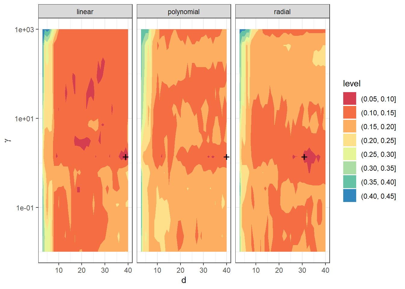
Figure 5.40: Dependency of validation error on the choice of hyperparameters \(d\) and \(\gamma\), separately for all three considered kernels in the SVM method.
Since we have already found the optimal values for the hyperparameters, we can construct the final models and determine their classification success on the test data.
Code
Code
# Prepare a data frame to store results
Res <- data.frame(model = c('SVM linear - RKHS - radial',
                            'SVM poly - RKHS - radial',
                            'SVM rbf - RKHS - radial'),
                  Err.train = NA,
                  Err.test = NA)

# Iterate through individual kernels
for (kernel_number in 1:3) {
  # Calculate the K matrix
  gamma <- gamma.opt[kernel_number] # Gamma value from CV
  K <- Kernel.RKHS(t.seq, gamma = gamma)

  # Determine eigenvalues and eigenvectors
  Eig <- eigen(K)
  eig.vals <- Eig$values
  eig.vectors <- Eig$vectors

  # Determine the alpha coefficients from SVM
  alpha.RKHS <- matrix(0, nrow = dim(data.RKHS)[1],
                       ncol = dim(data.RKHS)[2]) # Empty object

  # Model
  for(i in 1:dim(data.RKHS)[2]) {
    df.svm <- data.frame(x = t.seq,
                         y = data.RKHS[, i])
    svm.RKHS <- svm(y ~ x, data = df.svm,
                    kernel = 'radial',
                    type = 'eps-regression',
                    epsilon = 0.1,
                    gamma = gamma)
    # Determine alpha
    alpha.RKHS[svm.RKHS$index, i] <- svm.RKHS$coefs # Replace zeros with coefficients
  }

  # d
  d.RKHS <- d.opt[kernel_number]

  # Determine the lambda vector
  Lambda.RKHS <- matrix(NA,
                        ncol = dim(data.RKHS)[2],
                        nrow = d.RKHS) # Create empty object

  # Compute representation
  for(l in 1:dim(data.RKHS)[2]) {
    Lambda.RKHS[, l] <- (t(eig.vectors[, 1:d.RKHS]) %*% alpha.RKHS[, l]) * eig.vals[1:d.RKHS]
  }

  # Split into training and testing data
  XX.train <- Lambda.RKHS[, 1:dim(grid.data)[1]]
  XX.test <- Lambda.RKHS[, (dim(grid.data)[1] + 1):dim(Lambda.RKHS)[2]]

  kernel_type <- c('linear', 'polynomial', 'radial')[kernel_number]

  data.RKHS.train <- as.data.frame(t(XX.train))
  data.RKHS.train$Y <- factor(Y.train)

  data.RKHS.test <- as.data.frame(t(XX.test))
  data.RKHS.test$Y <- factor(Y.test)

  # Construct models
  clf.SVM.RKHS <- svm(Y ~ ., data = data.RKHS.train,
                      type = 'C-classification',
                      scale = TRUE,
                      coef0 = 1,
                      kernel = kernel_type)

  # Accuracy on training data
  predictions.train <- predict(clf.SVM.RKHS, newdata = data.RKHS.train)
  presnost.train <- table(Y.train, predictions.train) |>
    prop.table() |> diag() |> sum()

  # Accuracy on testing data
  predictions.test <- predict(clf.SVM.RKHS, newdata = data.RKHS.test)
  presnost.test <- table(Y.test, predictions.test) |>
    prop.table() |> diag() |> sum()

  # Store results
  Res[kernel_number, c(2, 3)] <- 1 - c(presnost.train, presnost.test)
}| Model | \(\widehat{Err}_{train}\quad\quad\quad\quad\quad\) | \(\widehat{Err}_{test}\quad\quad\quad\quad\quad\) |
|---|---|---|
| SVM linear - RKHS - radial | 0.0000 | 0.1833 |
| SVM poly - RKHS - radial | 0.0000 | 0.1500 |
| SVM rbf - RKHS - radial | 0.0214 | 0.1000 |
The error rate of the SVM method combined with the projection on the Reproducing Kernel Hilbert Space is thus equal to 0 % for the linear kernel, 0 % for the polynomial kernel, and 2.14 % for the Gaussian kernel on the training data. On the testing data, the error rate of the method is 18.33 % for the linear kernel, 15 % for the polynomial kernel, and 10 % for the radial kernel.
5.2.3.7.6.3 Polynomial Kernel
Code
# Remove the last column containing Y values
data.RKHS <- grid.data[, -dim(grid.data)[2]] |> t()
# Include test data as well
data.RKHS <- cbind(data.RKHS, grid.data.test[, -dim(grid.data.test)[2]] |> t())

# Kernel and kernel matrix ... polynomial with parameter p
Poly.kernel <- function(x, y, p) {
  return((1 + x * y)^p)
}

Kernel.RKHS <- function(x, p) {
  K <- matrix(NA, ncol = length(x), nrow = length(x))
  for(i in 1:nrow(K)) {
    for(j in 1:ncol(K)) {
      K[i, j] <- Poly.kernel(x = x[i], y = x[j], p)
    }
  }
  return(K)
}
Code
# Split training data into k parts
folds <- createMultiFolds(1:sum(split), k = k_cv, time = 1)
# Remove the last column containing Y values
data.RKHS <- grid.data[, -dim(grid.data)[2]] |> t()

# Hyperparameter values to iterate over
dimensions <- 3:40 # Reasonable range of d values
poly.cv <- 2:5

# List with three components ... array for individual kernels -> linear, poly, radial
# Empty matrix to insert individual results
# Columns will hold accuracy values for given parameters
# Rows will hold values for given p and layers corresponding to folds
dim.names <- list(p = paste0('p:', poly.cv),
                  d = paste0('d:', dimensions),
                  CV = paste0('cv:', 1:k_cv))

CV.results <- list(
  SVM.l = array(NA, dim = c(length(poly.cv), length(dimensions), k_cv),
                dimnames = dim.names),
  SVM.p = array(NA, dim = c(length(poly.cv), length(dimensions), k_cv),
                dimnames = dim.names),
  SVM.r = array(NA, dim = c(length(poly.cv), length(dimensions), k_cv),
                dimnames = dim.names))
Code
# Cross-validation
for (p in poly.cv) {
  K <- Kernel.RKHS(t.seq, p = p)
  Eig <- eigen(K)
  eig.vals <- Eig$values
  eig.vectors <- Eig$vectors
  alpha.RKHS <- matrix(0, nrow = dim(data.RKHS)[1], ncol = dim(data.RKHS)[2])

  # Model
  for(i in 1:dim(data.RKHS)[2]) {
    df.svm <- data.frame(x = t.seq,
                         y = data.RKHS[, i])
    svm.RKHS <- svm(y ~ x, data = df.svm,
                    kernel = 'polynomial',
                    type = 'eps-regression',
                    epsilon = 0.1,
                    coef0 = 1,
                    degree = p)
    alpha.RKHS[svm.RKHS$index, i] <- svm.RKHS$coefs
  }

  # Iterate through dimensions
  for(d.RKHS in dimensions) {
    Lambda.RKHS <- matrix(NA,
                          ncol = dim(data.RKHS)[2],
                          nrow = d.RKHS)
    # Compute representation
    for(l in 1:dim(data.RKHS)[2]) {
      Lambda.RKHS[, l] <- (t(eig.vectors[, 1:d.RKHS]) %*%
                             alpha.RKHS[, l]) * eig.vals[1:d.RKHS]
    }
    # Iterate through folds
    for (index_cv in 1:k_cv) {
      # Define test and training portions for CV
      fold <- folds[[index_cv]]
      # Split into training and validation data
      XX.train <- Lambda.RKHS[, fold]
      XX.test <- Lambda.RKHS[, !(1:dim(Lambda.RKHS)[2] %in% fold)]
      # Prepare a data frame to store results
      Res <- data.frame(model = c('SVM linear - RKHS',
                                  'SVM poly - RKHS',
                                  'SVM rbf - RKHS'),
                        Err.test = NA)
      # Iterate through individual kernels
      for (kernel_number in 1:3) {
        kernel_type <- c('linear', 'polynomial', 'radial')[kernel_number]

        data.RKHS.train <- as.data.frame(t(XX.train))
        data.RKHS.train$Y <- factor(Y.train[fold])

        data.RKHS.test <- as.data.frame(t(XX.test))
        data.RKHS.test$Y <- factor(Y.train[!(1:dim(Lambda.RKHS)[2] %in% fold)])

        # Construct models
        clf.SVM.RKHS <- svm(Y ~ ., data = data.RKHS.train,
                            type = 'C-classification',
                            scale = TRUE,
                            coef0 = 1,
                            kernel = kernel_type)

        # Accuracy on validation data
        predictions.test <- predict(clf.SVM.RKHS, newdata = data.RKHS.test)
        presnost.test <- table(data.RKHS.test$Y, predictions.test) |>
          prop.table() |> diag() |> sum()

        # Store results
        Res[kernel_number, 2] <- 1 - presnost.test
      }
      # Store accuracies in positions for given d, gamma, and fold
      CV.results$SVM.l[paste0('p:', p),
                       d.RKHS - min(dimensions) + 1,
                       index_cv] <- Res[1, 2]
      CV.results$SVM.p[paste0('p:', p),
                       d.RKHS - min(dimensions) + 1,
                       index_cv] <- Res[2, 2]
      CV.results$SVM.r[paste0('p:', p),
                       d.RKHS - min(dimensions) + 1,
                       index_cv] <- Res[3, 2]
    }
  }
}
Code
# Calculate average accuracies for each d across folds
for (n_method in 1:length(CV.results)) {
  CV.results[[n_method]] <- apply(CV.results[[n_method]], c(1, 2), mean)
}

poly.opt <- c(which.min(CV.results$SVM.l) %% length(poly.cv),
               which.min(CV.results$SVM.p) %% length(poly.cv),
               which.min(CV.results$SVM.r) %% length(poly.cv))
poly.opt[poly.opt == 0] <- length(poly.cv)
poly.opt <- poly.cv[poly.opt]

d.opt <- c(which.min(t(CV.results$SVM.l)) %% length(dimensions),
           which.min(t(CV.results$SVM.p)) %% length(dimensions),
           which.min(t(CV.results$SVM.r)) %% length(dimensions))
d.opt[d.opt == 0] <- length(dimensions)
d.opt <- dimensions[d.opt]

err.opt.cv <- c(min(CV.results$SVM.l),
                 min(CV.results$SVM.p),
                 min(CV.results$SVM.r))
df.RKHS.res <- data.frame(d = d.opt, p = poly.opt, CV = err.opt.cv,
                           Kernel = c('linear', 'polynomial', 'radial') |> factor(),
row.names = c('linear', 'poly', 'radial'))| \(\quad\quad\quad\quad\quad d\) | \(\quad\quad\quad\quad\quad p\) | \(\widehat{Err}_{cross\_validation}\) | Model | |
|---|---|---|---|---|
| linear | 20 | 2 | 0.0967 | linear |
| poly | 17 | 4 | 0.1119 | polynomial |
| radial | 22 | 5 | 0.1248 | radial |
We see that the best values for parameter \(d={}\) 20 and \(p={}\) 2 are for the linear kernel with an error calculated using 10-fold CV 0.0967, \(d={}\) 17 and \(p={}\) 4 for the polynomial kernel with an error calculated using 10-fold CV 0.1119, and \(d={}\) 22 and \(p={}\) 5 for the radial kernel with an error 0.1248.
Since we have found the optimal values for the hyperparameters, we can construct the final models and determine their classification success on the test data.
Code
Code
# Prepare a data frame to store results
Res <- data.frame(model = c('SVM linear - RKHS - poly',
                             'SVM poly - RKHS - poly',
                             'SVM rbf - RKHS - poly'),
                  Err.train = NA,
                  Err.test = NA)

# Iterate over the individual kernels
for (kernel_number in 1:3) {
  # Calculate the matrix K
  p <- poly.opt[kernel_number] # CV-derived parameter value
  K <- Kernel.RKHS(t.seq, p = p)

  # Determine eigenvalues and eigenvectors
  Eig <- eigen(K)
  eig.vals <- Eig$values
  eig.vectors <- Eig$vectors
  # Determine coefficients alpha from SVM
  alpha.RKHS <- matrix(0, nrow = dim(data.RKHS)[1],
                       ncol = dim(data.RKHS)[2]) # empty object

  # Model fitting
  for(i in 1:dim(data.RKHS)[2]) {
    df.svm <- data.frame(x = t.seq,
                         y = data.RKHS[, i])
    svm.RKHS <- svm(y ~ x, data = df.svm,
                    kernel = 'polynomial',
                    type = 'eps-regression',
                    epsilon = 0.1,
                    coef0 = 1,
                    degree = p)
    # Determine alpha
    alpha.RKHS[svm.RKHS$index, i] <- svm.RKHS$coefs # replace zeros with coefficients
  }
  # d
  d.RKHS <- d.opt[kernel_number]

  # Determine lambda vector
  Lambda.RKHS <- matrix(NA,
                        ncol = dim(data.RKHS)[2],
                        nrow = d.RKHS) # create empty object

  # Calculate representation
  for(l in 1:dim(data.RKHS)[2]) {
    Lambda.RKHS[, l] <- (t(eig.vectors[, 1:d.RKHS]) %*% alpha.RKHS[, l]) * eig.vals[1:d.RKHS]
  }

  # Split into training and test data
  XX.train <- Lambda.RKHS[, 1:dim(grid.data)[1]]
  XX.test <- Lambda.RKHS[, (dim(grid.data)[1] + 1):dim(Lambda.RKHS)[2]]

  kernel_type <- c('linear', 'polynomial', 'radial')[kernel_number]

  data.RKHS.train <- as.data.frame(t(XX.train))
  data.RKHS.train$Y <- factor(Y.train)

  data.RKHS.test <- as.data.frame(t(XX.test))
  data.RKHS.test$Y <- factor(Y.test)

  # Build the models
  clf.SVM.RKHS <- svm(Y ~ ., data = data.RKHS.train,
                      type = 'C-classification',
                      scale = TRUE,
                      coef0 = 1,
                      kernel = kernel_type)

  # Accuracy on training data
  predictions.train <- predict(clf.SVM.RKHS, newdata = data.RKHS.train)
  presnost.train <- table(Y.train, predictions.train) |>
    prop.table() |> diag() |> sum()

  # Accuracy on test data
  predictions.test <- predict(clf.SVM.RKHS, newdata = data.RKHS.test)
  presnost.test <- table(Y.test, predictions.test) |>
    prop.table() |> diag() |> sum()

  # Store results
  Res[kernel_number, c(2, 3)] <- 1 - c(presnost.train, presnost.test)
}| Model | \(\widehat{Err}_{train}\quad\quad\quad\quad\quad\) | \(\widehat{Err}_{test}\quad\quad\quad\quad\quad\) |
|---|---|---|
| SVM linear - RKHS - poly | 0.0643 | 0.2333 |
| SVM poly - RKHS - poly | 0.0643 | 0.1167 |
| SVM rbf - RKHS - poly | 0.0929 | 0.1333 |
The error rate of the SVM method combined with projection onto the Reproducing Kernel Hilbert Space is thus on the training data equal to 6.43 % for the linear kernel, 6.43 % for the polynomial kernel, and 9.29 % for the Gaussian kernel. On the test data, the error rate of the method is 23.33 % for the linear kernel, 11.67 % for the polynomial kernel, and 13.33 % for the radial kernel.
5.2.3.7.6.4 Linear Kernel
Code
# Remove the last column, which contains the Y values
data.RKHS <- grid.data[, -dim(grid.data)[2]] |> t()
# Add the test data as well
data.RKHS <- cbind(data.RKHS, grid.data.test[, -dim(grid.data.test)[2]] |> t())

# Kernel and kernel matrix ... polynomial with parameter p
Linear.kernel <- function(x, y) {
  return(x * y)
}

Kernel.RKHS <- function(x) {
  K <- matrix(NA, ncol = length(x), nrow = length(x))
  for(i in 1:nrow(K)) {
    for(j in 1:ncol(K)) {
      K[i, j] <- Linear.kernel(x = x[i], y = x[j])
    }
  }
  return(K)
}
Code
# Split the training data into k parts
folds <- createMultiFolds(1:sum(split), k = k_cv, time = 1)
# Remove the last column, which contains the Y values
data.RKHS <- grid.data[, -dim(grid.data)[2]] |> t()

# Values of hyperparameters that we will traverse
dimensions <- 3:40 # Reasonable range of values for d

# List with three components ... array for individual kernels -> linear, poly, radial
# Empty matrix to store the individual results
# In columns, there will be accuracy values for given d
# In rows, there will be values for layers corresponding to folds
dim.names <- list(d = paste0('d:', dimensions),
                  CV = paste0('cv:', 1:k_cv))

CV.results <- list(
  SVM.l = array(NA, dim = c(length(dimensions), k_cv),
                dimnames = dim.names),
  SVM.p = array(NA, dim = c(length(dimensions), k_cv),
                dimnames = dim.names),
  SVM.r = array(NA, dim = c(length(dimensions), k_cv),
                dimnames = dim.names))
Code
# Cross-validation
K <- Kernel.RKHS(t.seq)
Eig <- eigen(K)
eig.vals <- Eig$values
eig.vectors <- Eig$vectors
alpha.RKHS <- matrix(0, nrow = dim(data.RKHS)[1], ncol = dim(data.RKHS)[2])

# Model
for(i in 1:dim(data.RKHS)[2]) {
  df.svm <- data.frame(x = t.seq,
                       y = data.RKHS[, i])
  svm.RKHS <- svm(y ~ x, data = df.svm,
                  kernel = 'linear',
                  type = 'eps-regression',
                  epsilon = 0.1)
  alpha.RKHS[svm.RKHS$index, i] <- svm.RKHS$coefs
}

# Traverse dimensions
for(d.RKHS in dimensions) {
  Lambda.RKHS <- matrix(NA,
                        ncol = dim(data.RKHS)[2],
                        nrow = d.RKHS)
  # Calculation of representation
  for(l in 1:dim(data.RKHS)[2]) {
    Lambda.RKHS[, l] <- (t(eig.vectors[, 1:d.RKHS]) %*%
                           alpha.RKHS[, l]) * eig.vals[1:d.RKHS]
  }
  # Traverse folds
  for (index_cv in 1:k_cv) {
    # Define test and training portions for CV
    fold <- folds[[index_cv]]
    # Split into training and validation data
    XX.train <- Lambda.RKHS[, fold]
    XX.test <- Lambda.RKHS[, !(1:dim(Lambda.RKHS)[2] %in% fold)]
    # Prepare a data table to store results
    Res <- data.frame(model = c('SVM linear - RKHS',
                                'SVM poly - RKHS',
                                'SVM rbf - RKHS'),
                      Err.test = NA)
    # Traverse individual kernels
    for (kernel_number in 1:3) {
      kernel_type <- c('linear', 'polynomial', 'radial')[kernel_number]

      data.RKHS.train <- as.data.frame(t(XX.train))
      data.RKHS.train$Y <- factor(Y.train[fold])

      data.RKHS.test <- as.data.frame(t(XX.test))
      data.RKHS.test$Y <- factor(Y.train[!(1:dim(Lambda.RKHS)[2] %in% fold)])

      # Build models
      clf.SVM.RKHS <- svm(Y ~ ., data = data.RKHS.train,
                          type = 'C-classification',
                          scale = TRUE,
                          coef0 = 1,
                          kernel = kernel_type)

      # Accuracy on validation data
      predictions.test <- predict(clf.SVM.RKHS, newdata = data.RKHS.test)
      accuracy.test <- table(data.RKHS.test$Y, predictions.test) |>
        prop.table() |> diag() |> sum()

      # Store results
      Res[kernel_number, 2] <- 1 - accuracy.test
    }
    # Store accuracies in positions for given d, gamma, and fold
    CV.results$SVM.l[d.RKHS - min(dimensions) + 1,
                     index_cv] <- Res[1, 2]
    CV.results$SVM.p[d.RKHS - min(dimensions) + 1,
                     index_cv] <- Res[2, 2]
    CV.results$SVM.r[d.RKHS - min(dimensions) + 1,
                     index_cv] <- Res[3, 2]
  }
}
Code
# Calculate average accuracies for each d across folds
for (n_method in 1:length(CV.results)) {
  CV.results[[n_method]] <- apply(CV.results[[n_method]], 1, mean)
}

d.opt <- c(which.min(t(CV.results$SVM.l)) %% length(dimensions),
           which.min(t(CV.results$SVM.p)) %% length(dimensions),
           which.min(t(CV.results$SVM.r)) %% length(dimensions))
d.opt[d.opt == 0] <- length(dimensions)
d.opt <- dimensions[d.opt]

err.opt.cv <- c(min(CV.results$SVM.l),
                     min(CV.results$SVM.p),
                     min(CV.results$SVM.r))
df.RKHS.res <- data.frame(d = d.opt, CV = err.opt.cv,
           Kernel = c('linear', 'polynomial', 'radial') |> factor(),
row.names = c('linear', 'poly', 'radial'))| \(\quad\quad\quad\quad\quad d\) | \(\widehat{Err}_{cross\_validation}\) | Model | |
|---|---|---|---|
| linear | 14 | 0.1509 | linear |
| poly | 16 | 0.1642 | polynomial |
| radial | 36 | 0.1510 | radial |
We see that the optimal parameter value is \(d={}\) 14 for the linear kernel with an error rate calculated using 10-fold CV of 0.1509, \(d={}\) 16 for the polynomial kernel with an error rate of 0.1642, and \(d={}\) 36 for the radial kernel with an error rate of 0.151.
Now that we have found the optimal hyperparameter values, we can construct the final models and determine their classification success on the test data.
Code
Code
# Prepare a data frame to store the results
Res <- data.frame(model = c('SVM linear - RKHS - linear',
                            'SVM poly - RKHS - linear',
                            'SVM rbf - RKHS - linear'),
                  Err.train = NA,
                  Err.test = NA)

# Iterate over the individual kernels
for (kernel_number in 1:3) {
  # Compute the K matrix
  K <- Kernel.RKHS(t.seq)

  # Determine eigenvalues and eigenvectors
  Eig <- eigen(K)
  eig.vals <- Eig$values
  eig.vectors <- Eig$vectors
  # Determine alpha coefficients from SVM
  alpha.RKHS <- matrix(0, nrow = dim(data.RKHS)[1],
                       ncol = dim(data.RKHS)[2]) # empty object

  # Model
  for(i in 1:dim(data.RKHS)[2]) {
    df.svm <- data.frame(x = t.seq,
                         y = data.RKHS[, i])
    svm.RKHS <- svm(y ~ x, data = df.svm,
                    kernel = 'linear',
                    type = 'eps-regression',
                    epsilon = 0.1)
    # Determine alpha
    alpha.RKHS[svm.RKHS$index, i] <- svm.RKHS$coefs # replace zeros with coefficients
  }
  # d
  d.RKHS <- d.opt[kernel_number]

  # Determine lambda vector
  Lambda.RKHS <- matrix(NA,
                        ncol = dim(data.RKHS)[2],
                        nrow = d.RKHS) # create empty object

  # Calculate representation
  for(l in 1:dim(data.RKHS)[2]) {
    Lambda.RKHS[, l] <- (t(eig.vectors[, 1:d.RKHS]) %*% alpha.RKHS[, l]) * eig.vals[1:d.RKHS]
  }

  # Split into training and test data
  XX.train <- Lambda.RKHS[, 1:dim(grid.data)[1]]
  XX.test <- Lambda.RKHS[, (dim(grid.data)[1] + 1):dim(Lambda.RKHS)[2]]

  kernel_type <- c('linear', 'polynomial', 'radial')[kernel_number]

  data.RKHS.train <- as.data.frame(t(XX.train))
  data.RKHS.train$Y <- factor(Y.train)

  data.RKHS.test <- as.data.frame(t(XX.test))
  data.RKHS.test$Y <- factor(Y.test)

  # Build the model
  clf.SVM.RKHS <- svm(Y ~ ., data = data.RKHS.train,
                      type = 'C-classification',
                      scale = TRUE,
                      coef0 = 1,
                      kernel = kernel_type)

  # Accuracy on training data
  predictions.train <- predict(clf.SVM.RKHS, newdata = data.RKHS.train)
  accuracy.train <- table(Y.train, predictions.train) |>
    prop.table() |> diag() |> sum()

  # Accuracy on test data
  predictions.test <- predict(clf.SVM.RKHS, newdata = data.RKHS.test)
  accuracy.test <- table(Y.test, predictions.test) |>
    prop.table() |> diag() |> sum()

  # Store the results
  Res[kernel_number, c(2, 3)] <- 1 - c(accuracy.train, accuracy.test)
}| Model | \(\widehat{Err}_{train}\quad\quad\quad\quad\quad\) | \(\widehat{Err}_{test}\quad\quad\quad\quad\quad\) |
|---|---|---|
| SVM linear - RKHS - linear | 0.1214 | 0.2333 |
| SVM poly - RKHS - linear | 0.0571 | 0.2167 |
| SVM rbf - RKHS - linear | 0.0714 | 0.1500 |
The error rate of the SVM method combined with projection onto the Reproducing Kernel Hilbert Space is thus 12.14 % for the linear kernel, 5.71 % for the polynomial kernel, and 7.14 % for the Gaussian kernel. For the test data, the error rate is 23.33 % for the linear kernel, 21.67 % for the polynomial kernel, and 15 % for the radial kernel.
5.2.3.8 Results Table
| Model | \(\widehat{Err}_{train}\quad\quad\quad\quad\quad\) | \(\widehat{Err}_{test}\quad\quad\quad\quad\quad\) |
|---|---|---|
| KNN | 0.1500 | 0.1500 |
| LDA | 0.1357 | 0.1833 |
| QDA | 0.1429 | 0.1500 |
| LR functional | 0.0429 | 0.0833 |
| LR score | 0.1357 | 0.1833 |
| Tree - discr. | 0.0857 | 0.1500 |
| Tree - score | 0.1643 | 0.2833 |
| Tree - Bbasis | 0.1000 | 0.1167 |
| RForest - discretization | 0.0071 | 0.1333 |
| RForest - score | 0.0286 | 0.2000 |
| RForest - Bbasis | 0.0071 | 0.1000 |
| SVM linear - func | 0.0786 | 0.0833 |
| SVM poly - func | 0.0714 | 0.1000 |
| SVM rbf - func | 0.0571 | 0.0833 |
| SVM linear - discr | 0.0929 | 0.1000 |
| SVM poly - discr | 0.0929 | 0.1000 |
| SVM rbf - discr | 0.0643 | 0.1000 |
| SVM linear - PCA | 0.1357 | 0.1833 |
| SVM poly - PCA | 0.1286 | 0.1833 |
| SVM rbf - PCA | 0.1357 | 0.1667 |
| SVM linear - Bbasis | 0.0571 | 0.0667 |
| SVM poly - Bbasis | 0.0929 | 0.0667 |
| SVM rbf - Bbasis | 0.0143 | 0.0833 |
| SVM linear - projection | 0.0500 | 0.0833 |
| SVM poly - projection | 0.0286 | 0.1167 |
| SVM rbf - projection | 0.0500 | 0.0833 |
| SVM linear - RKHS - radial | 0.0000 | 0.1833 |
| SVM poly - RKHS - radial | 0.0000 | 0.1500 |
| SVM rbf - RKHS - radial | 0.0214 | 0.1000 |
| SVM linear - RKHS - poly | 0.0643 | 0.2333 |
| SVM poly - RKHS - poly | 0.0643 | 0.1167 |
| SVM rbf - RKHS - poly | 0.0929 | 0.1333 |
| SVM linear - RKHS - linear | 0.1214 | 0.2333 |
| SVM poly - RKHS - linear | 0.0571 | 0.2167 |
| SVM rbf - RKHS - linear | 0.0714 | 0.1500 |
5.2.4 Simulation Study
In the entire previous section, we dealt with only one randomly generated set of functions from two classification classes, which we subsequently divided randomly into test and training parts.
Then we evaluated each classifier obtained by the considered methods based on the test and training error rates.
Since the generated data (and their division into two parts) may vary significantly with each repetition, the error rates of the individual classification algorithms will also vary considerably.
Therefore, drawing any conclusions about the methods and comparing them with each other based on a single generated dataset can be very misleading.
For this reason, in this section, we will focus on repeating the entire previous procedure for different generated datasets.
We will store the results in a table and, in the end, calculate the average model characteristics across the individual repetitions.
To ensure our conclusions are sufficiently general, we will choose the number of repetitions \(n_{sim} = 100\).
Code
# Setting the pseudorandom number generator
set.seed(42)
# Number of simulations
n.sim <- 100
## List to store error rates
# Columns represent methods
# Rows represent individual repetitions
# The list has two items ... train and test
methods <- c('KNN', 'LDA', 'QDA', 'LR_functional', 'LR_score', 'Tree_discr',
'Tree_score', 'Tree_Bbasis', 'RF_discr', 'RF_score', 'RF_Bbasis',
'SVM linear - func', 'SVM poly - func', 'SVM rbf - func',
'SVM linear - diskr', 'SVM poly - diskr', 'SVM rbf - diskr',
'SVM linear - PCA', 'SVM poly - PCA', 'SVM rbf - PCA',
'SVM linear - Bbasis', 'SVM poly - Bbasis', 'SVM rbf - Bbasis',
'SVM linear - projection', 'SVM poly - projection',
'SVM rbf - projection', 'SVM linear - RKHS - radial',
'SVM poly - RKHS - radial', 'SVM rbf - RKHS - radial',
'SVM linear - RKHS - poly', 'SVM poly - RKHS - poly',
'SVM rbf - RKHS - poly', 'SVM linear - RKHS - linear',
'SVM poly - RKHS - linear', 'SVM rbf - RKHS - linear')
SIMULACE <- list(train = as.data.frame(matrix(NA, ncol = length(methods),
nrow = n.sim,
dimnames = list(1:n.sim, methods))),
test = as.data.frame(matrix(NA, ncol = length(methods),
nrow = n.sim,
dimnames = list(1:n.sim, methods))))
# Object to store optimal hyperparameter values, determined by CV
CV_RESULTS <- data.frame(KNN_K = rep(NA, n.sim),
nharm = NA,
LR_func_n_basis = NA,
SVM_d_Linear = NA,
SVM_d_Poly = NA,
SVM_d_Radial = NA,
SVM_RKHS_radial_gamma1 = NA,
SVM_RKHS_radial_gamma2 = NA,
SVM_RKHS_radial_gamma3 = NA,
SVM_RKHS_radial_d1 = NA,
SVM_RKHS_radial_d2 = NA,
SVM_RKHS_radial_d3 = NA,
SVM_RKHS_poly_p1 = NA,
SVM_RKHS_poly_p2 = NA,
SVM_RKHS_poly_p3 = NA,
SVM_RKHS_poly_d1 = NA,
SVM_RKHS_poly_d2 = NA,
SVM_RKHS_poly_d3 = NA,
SVM_RKHS_linear_d1 = NA,
SVM_RKHS_linear_d2 = NA,
SVM_RKHS_linear_d3 = NA)Now we will repeat the entire previous part 100 times, and we will store the error rate values in the list SIMULACE.
In the data table CV_RESULTS, we will store the optimal hyperparameter values—specifically for the \(K\)-nearest neighbors method and the SVM dimension \(d\) in the case of projection onto a B-spline basis.
We will also save all hyperparameter values for the SVM + RKHS method.
Code
# nastaveni generatoru pseudonahodnych cisel
set.seed(42)
## SIMULACE
for(sim in 1:n.sim) {
# pocet vygenerovanych pozorovani pro kazdou tridu
n <- 100
# vektor casu ekvidistantni na intervalu [0, 6]
t <- seq(0, 6, length = 51)
# pro Y = 0
X0 <- generate_values(t, funkce_0, n, 1, 2)
# pro Y = 1
X1 <- generate_values(t, funkce_1, n, 1, 2)
rangeval <- range(t)
breaks <- t
norder <- 6
bbasis <- create.bspline.basis(rangeval = rangeval,
norder = norder,
breaks = breaks)
curv.Lfd <- int2Lfd(4)
# spojeni pozorovani do jedne matice
XX <- cbind(X0, X1)
lambda.vect <- 10^seq(from = -4.5, to = -1.5, length.out = 25) # vektor lambd
gcv <- rep(NA, length = length(lambda.vect)) # prazdny vektor pro ulozebi GCV
for(index in 1:length(lambda.vect)) {
curv.Fdpar <- fdPar(bbasis, curv.Lfd, lambda.vect[index])
BSmooth <- smooth.basis(t, XX, curv.Fdpar) # vyhlazeni
gcv[index] <- mean(BSmooth$gcv) # prumer pres vsechny pozorovane krivky
}
GCV <- data.frame(
lambda = round(log10(lambda.vect), 3),
GCV = gcv
)
# najdeme hodnotu minima
lambda.opt <- lambda.vect[which.min(gcv)]
curv.fdPar <- fdPar(bbasis, curv.Lfd, lambda.opt)
BSmooth <- smooth.basis(t, XX, curv.fdPar)
XXfd <- BSmooth$fd
# vypocet derivace
XXder <- deriv.fd(XXfd, 2)
fdobjSmootheval <- eval.fd(fdobj = XXder, evalarg = t)
# rozdeleni na testovaci a trenovaci cast
split <- sample.split(XXder$fdnames$reps, SplitRatio = 0.7)
Y <- rep(c(0, 1), each = n)
X.train <- subset(XXder, split == TRUE)
X.test <- subset(XXder, split == FALSE)
Y.train <- subset(Y, split == TRUE)
Y.test <- subset(Y, split == FALSE)
x.train <- fdata(X.train)
y.train <- as.numeric(factor(Y.train))
## 1) K nejbližších sousedů
k_cv <- 10 # k-fold CV
neighbours <- 1:20 #c(1:(2 * ceiling(sqrt(length(y.train))))) # pocet sousedu
# rozdelime trenovaci data na k casti
folds <- createMultiFolds(X.train$fdnames$reps, k = k_cv, time = 1)
CV.results <- matrix(NA, nrow = length(neighbours), ncol = k_cv)
for (index in 1:k_cv) {
# definujeme danou indexovou mnozinu
fold <- folds[[index]]
x.train.cv <- subset(X.train, c(1:length(X.train$fdnames$reps)) %in% fold) |>
fdata()
y.train.cv <- subset(Y.train, c(1:length(X.train$fdnames$reps)) %in% fold) |>
factor() |> as.numeric()
x.test.cv <- subset(X.train, !c(1:length(X.train$fdnames$reps)) %in% fold) |>
fdata()
y.test.cv <- subset(Y.train, !c(1:length(X.train$fdnames$reps)) %in% fold) |>
factor() |> as.numeric()
# projdeme kazdou cast ... k-krat zopakujeme
for(neighbour in neighbours) {
# model pro konkretni volbu K
neighb.model <- classif.knn(group = y.train.cv,
fdataobj = x.train.cv,
knn = neighbour)
# predikce na validacni casti
model.neighb.predict <- predict(neighb.model,
new.fdataobj = x.test.cv)
# presnost na validacni casti
presnost <- table(y.test.cv, model.neighb.predict) |>
prop.table() |> diag() |> sum()
# presnost vlozime na pozici pro dane K a fold
CV.results[neighbour, index] <- presnost
}
}
# spocitame prumerne presnosti pro jednotliva K pres folds
CV.results <- apply(CV.results, 1, mean)
K.opt <- which.max(CV.results)
CV_RESULTS$KNN_K[sim] <- K.opt
presnost.opt.cv <- max(CV.results)
CV.results <- data.frame(K = neighbours, CV = CV.results)
neighb.model <- classif.knn(group = y.train, fdataobj = x.train, knn = K.opt)
# predikce
model.neighb.predict <- predict(neighb.model,
new.fdataobj = fdata(X.test))
presnost <- table(as.numeric(factor(Y.test)), model.neighb.predict) |>
prop.table() |>
diag() |>
sum()
RESULTS <- data.frame(model = 'KNN',
Err.train = 1 - neighb.model$max.prob,
Err.test = 1 - presnost)
## 2) Lineární diskriminační analýza
# analyza hlavnich komponent
data.PCA <- pca.fd(X.train, nharm = 10) # nharm - maximalni pocet HK
nharm <- which(cumsum(data.PCA$varprop) >= 0.9)[1] # urceni p
CV_RESULTS$nharm[sim] <- nharm
if(nharm == 1) nharm <- 2
data.PCA <- pca.fd(X.train, nharm = nharm)
data.PCA.train <- as.data.frame(data.PCA$scores) # skore prvnich p HK
data.PCA.train$Y <- factor(Y.train) # prislusnost do trid
# vypocet skoru testovacich funkci
scores <- matrix(NA, ncol = nharm, nrow = length(Y.test)) # prazdna matice
for(k in 1:dim(scores)[1]) {
xfd = X.test[k] - data.PCA$meanfd[1] # k-te pozorovani - prumerna funkce
scores[k, ] = inprod(xfd, data.PCA$harmonics)
# skalarni soucin rezidua a vlastnich funkci rho (funkcionalni hlavni komponenty)
}
data.PCA.test <- as.data.frame(scores)
data.PCA.test$Y <- factor(Y.test)
colnames(data.PCA.test) <- colnames(data.PCA.train)
# model
clf.LDA <- lda(Y ~ ., data = data.PCA.train)
# presnost na trenovacich datech
predictions.train <- predict(clf.LDA, newdata = data.PCA.train)
presnost.train <- table(data.PCA.train$Y, predictions.train$class) |>
prop.table() |> diag() |> sum()
# presnost na trenovacich datech
predictions.test <- predict(clf.LDA, newdata = data.PCA.test)
presnost.test <- table(data.PCA.test$Y, predictions.test$class) |>
prop.table() |> diag() |> sum()
Res <- data.frame(model = 'LDA',
Err.train = 1 - presnost.train,
Err.test = 1 - presnost.test)
RESULTS <- rbind(RESULTS, Res)
## 3) Kvadratická diskriminační analýza
# model
clf.QDA <- qda(Y ~ ., data = data.PCA.train)
# presnost na trenovacich datech
predictions.train <- predict(clf.QDA, newdata = data.PCA.train)
presnost.train <- table(data.PCA.train$Y, predictions.train$class) |>
prop.table() |> diag() |> sum()
# presnost na trenovacich datech
predictions.test <- predict(clf.QDA, newdata = data.PCA.test)
presnost.test <- table(data.PCA.test$Y, predictions.test$class) |>
prop.table() |> diag() |> sum()
Res <- data.frame(model = 'QDA',
Err.train = 1 - presnost.train,
Err.test = 1 - presnost.test)
RESULTS <- rbind(RESULTS, Res)
## 4) Logistická regrese
### 4.1) Funkcionální logistická regrese
# vytvorime vhodne objekty
x.train <- fdata(X.train)
y.train <- as.numeric(Y.train)
# body, ve kterych jsou funkce vyhodnoceny
tt <- x.train[["argvals"]]
dataf <- as.data.frame(y.train)
colnames(dataf) <- "Y"
# B-spline baze
# basis1 <- X.train$basis
nbasis.x <- 20
rangeval <- range(tt)
norder <- 6
basis1 <- create.bspline.basis(rangeval = rangeval,
norder = norder,
nbasis = nbasis.x)
### 10-fold cross-validation
n.basis.max <- 15
n.basis <- 4:n.basis.max
k_cv <- 10 # k-fold CV
# rozdelime trenovaci data na k casti
folds <- createMultiFolds(X.train$fdnames$reps, k = k_cv, time = 1)
## prvky, ktere se behem cyklu nemeni
# body, ve kterych jsou funkce vyhodnoceny
tt <- x.train[["argvals"]]
# B-spline baze
# basis1 <- X.train$basis
basis1 <- create.bspline.basis(rangeval = rangeval,
norder = norder,
nbasis = 50)
# vztah
f <- Y ~ x
# baze pro x
basis.x <- list("x" = basis1)
CV.results <- matrix(NA, nrow = length(n.basis), ncol = k_cv,
dimnames = list(n.basis, 1:k_cv))
for (index in 1:k_cv) {
# definujeme danou indexovou mnozinu
fold <- folds[[index]]
x.train.cv <- subset(X.train, c(1:length(X.train$fdnames$reps)) %in% fold) |>
fdata()
y.train.cv <- subset(Y.train, c(1:length(X.train$fdnames$reps)) %in% fold) |>
as.numeric()
x.test.cv <- subset(X.train, !c(1:length(X.train$fdnames$reps)) %in% fold) |>
fdata()
y.test.cv <- subset(Y.train, !c(1:length(X.train$fdnames$reps)) %in% fold) |>
as.numeric()
dataf <- as.data.frame(y.train.cv)
colnames(dataf) <- "Y"
for (i in n.basis) {
# baze pro bety
basis2 <- create.bspline.basis(rangeval = rangeval, nbasis = i)
basis.b <- list("x" = basis2)
# vstupni data do modelu
ldata <- list("df" = dataf, "x" = x.train.cv)
# binomicky model ... model logisticke regrese
model.glm <- fregre.glm(f, family = binomial(), data = ldata,
basis.x = basis.x, basis.b = basis.b)
# presnost na validacni casti
newldata = list("df" = as.data.frame(y.test.cv), "x" = x.test.cv)
predictions.valid <- predict(model.glm, newx = newldata)
predictions.valid <- data.frame(Y.pred = ifelse(predictions.valid < 1/2, 0, 1))
presnost.valid <- table(y.test.cv, predictions.valid$Y.pred) |>
prop.table() |> diag() |> sum()
# vlozime do matice
CV.results[as.character(i), as.character(index)] <- presnost.valid
}
}
# spocitame prumerne presnosti pro jednotliva n pres folds
CV.results <- apply(CV.results, 1, mean)
n.basis.opt <- n.basis[which.max(CV.results)]
CV_RESULTS$LR_func_n_basis[sim] <- n.basis.opt
presnost.opt.cv <- max(CV.results)
# optimalni model
basis2 <- create.bspline.basis(rangeval = range(tt), nbasis = n.basis.opt)
f <- Y ~ x
# baze pro x a bety
basis.x <- list("x" = basis1)
basis.b <- list("x" = basis2)
# vstupni data do modelu
dataf <- as.data.frame(y.train)
colnames(dataf) <- "Y"
ldata <- list("df" = dataf, "x" = x.train)
# binomicky model ... model logisticke regrese
model.glm <- fregre.glm(f, family = binomial(), data = ldata,
basis.x = basis.x, basis.b = basis.b)
# presnost na trenovacich datech
predictions.train <- predict(model.glm, newx = ldata)
predictions.train <- data.frame(Y.pred = ifelse(predictions.train < 1/2, 0, 1))
presnost.train <- table(Y.train, predictions.train$Y.pred) |>
prop.table() |> diag() |> sum()
# presnost na trenovacich datech
newldata = list("df" = as.data.frame(Y.test), "x" = fdata(X.test))
predictions.test <- predict(model.glm, newx = newldata)
predictions.test <- data.frame(Y.pred = ifelse(predictions.test < 1/2, 0, 1))
presnost.test <- table(Y.test, predictions.test$Y.pred) |>
prop.table() |> diag() |> sum()
Res <- data.frame(model = 'LR_functional',
Err.train = 1 - presnost.train,
Err.test = 1 - presnost.test)
RESULTS <- rbind(RESULTS, Res)
### 4.2) Logistická regrese s analýzou hlavních komponent
# model
clf.LR <- glm(Y ~ ., data = data.PCA.train, family = binomial)
# presnost na trenovacich datech
predictions.train <- predict(clf.LR, newdata = data.PCA.train, type = 'response')
predictions.train <- ifelse(predictions.train > 0.5, 1, 0)
presnost.train <- table(data.PCA.train$Y, predictions.train) |>
prop.table() |> diag() |> sum()
# presnost na trenovacich datech
predictions.test <- predict(clf.LR, newdata = data.PCA.test, type = 'response')
predictions.test <- ifelse(predictions.test > 0.5, 1, 0)
presnost.test <- table(data.PCA.test$Y, predictions.test) |>
prop.table() |> diag() |> sum()
Res <- data.frame(model = 'LR_score',
Err.train = 1 - presnost.train,
Err.test = 1 - presnost.test)
RESULTS <- rbind(RESULTS, Res)
## 5) Rozhodovací stromy
### 5.1) Diskretizace intervalu
# posloupnost bodu, ve kterych funkce vyhodnotime
t.seq <- seq(0, 6, length = 101)
grid.data <- eval.fd(fdobj = X.train, evalarg = t.seq)
grid.data <- as.data.frame(t(grid.data)) # transpozice kvuli funkcim v radku
grid.data$Y <- Y.train |> factor()
grid.data.test <- eval.fd(fdobj = X.test, evalarg = t.seq)
grid.data.test <- as.data.frame(t(grid.data.test))
grid.data.test$Y <- Y.test |> factor()
# sestrojeni modelu
clf.tree <- train(Y ~ ., data = grid.data,
method = "rpart",
trControl = trainControl(method = "CV", number = 10),
metric = "Accuracy")
# presnost na trenovacich datech
predictions.train <- predict(clf.tree, newdata = grid.data)
presnost.train <- table(Y.train, predictions.train) |>
prop.table() |> diag() |> sum()
# presnost na trenovacich datech
predictions.test <- predict(clf.tree, newdata = grid.data.test)
presnost.test <- table(Y.test, predictions.test) |>
prop.table() |> diag() |> sum()
Res <- data.frame(model = 'Tree_discr',
Err.train = 1 - presnost.train,
Err.test = 1 - presnost.test)
RESULTS <- rbind(RESULTS, Res)
### 5.2) Skóre hlavních komponent
# sestrojeni modelu
clf.tree.PCA <- train(Y ~ ., data = data.PCA.train,
method = "rpart",
trControl = trainControl(method = "CV", number = 10),
metric = "Accuracy")
# presnost na trenovacich datech
predictions.train <- predict(clf.tree.PCA, newdata = data.PCA.train)
presnost.train <- table(Y.train, predictions.train) |>
prop.table() |> diag() |> sum()
# presnost na trenovacich datech
predictions.test <- predict(clf.tree.PCA, newdata = data.PCA.test)
presnost.test <- table(Y.test, predictions.test) |>
prop.table() |> diag() |> sum()
Res <- data.frame(model = 'Tree_score',
Err.train = 1 - presnost.train,
Err.test = 1 - presnost.test)
RESULTS <- rbind(RESULTS, Res)
### 5.3) Bázové koeficienty
# trenovaci dataset
data.Bbasis.train <- t(X.train$coefs) |> as.data.frame()
data.Bbasis.train$Y <- factor(Y.train)
# testovaci dataset
data.Bbasis.test <- t(X.test$coefs) |> as.data.frame()
data.Bbasis.test$Y <- factor(Y.test)
# sestrojeni modelu
clf.tree.Bbasis <- train(Y ~ ., data = data.Bbasis.train,
method = "rpart",
trControl = trainControl(method = "CV", number = 10),
metric = "Accuracy")
# presnost na trenovacich datech
predictions.train <- predict(clf.tree.Bbasis, newdata = data.Bbasis.train)
presnost.train <- table(Y.train, predictions.train) |>
prop.table() |> diag() |> sum()
# presnost na trenovacich datech
predictions.test <- predict(clf.tree.Bbasis, newdata = data.Bbasis.test)
presnost.test <- table(Y.test, predictions.test) |>
prop.table() |> diag() |> sum()
Res <- data.frame(model = 'Tree_Bbasis',
Err.train = 1 - presnost.train,
Err.test = 1 - presnost.test)
RESULTS <- rbind(RESULTS, Res)
## 6) Náhodné lesy
### 6.1) Diskretizace intervalu
# sestrojeni modelu
clf.RF <- randomForest(Y ~ ., data = grid.data,
ntree = 500, # pocet stromu
importance = TRUE,
nodesize = 5)
# presnost na trenovacich datech
predictions.train <- predict(clf.RF, newdata = grid.data)
presnost.train <- table(Y.train, predictions.train) |>
prop.table() |> diag() |> sum()
# presnost na trenovacich datech
predictions.test <- predict(clf.RF, newdata = grid.data.test)
presnost.test <- table(Y.test, predictions.test) |>
prop.table() |> diag() |> sum()
Res <- data.frame(model = 'RF_discr',
Err.train = 1 - presnost.train,
Err.test = 1 - presnost.test)
RESULTS <- rbind(RESULTS, Res)
### 6.2) Skóre hlavních komponent
# sestrojeni modelu
clf.RF.PCA <- randomForest(Y ~ ., data = data.PCA.train,
ntree = 500, # pocet stromu
importance = TRUE,
nodesize = 5)
# presnost na trenovacich datech
predictions.train <- predict(clf.RF.PCA, newdata = data.PCA.train)
presnost.train <- table(Y.train, predictions.train) |>
prop.table() |> diag() |> sum()
# presnost na trenovacich datech
predictions.test <- predict(clf.RF.PCA, newdata = data.PCA.test)
presnost.test <- table(Y.test, predictions.test) |>
prop.table() |> diag() |> sum()
Res <- data.frame(model = 'RF_score',
Err.train = 1 - presnost.train,
Err.test = 1 - presnost.test)
RESULTS <- rbind(RESULTS, Res)
### 6.3) Bázové koeficienty
# sestrojeni modelu
clf.RF.Bbasis <- randomForest(Y ~ ., data = data.Bbasis.train,
ntree = 500, # pocet stromu
importance = TRUE,
nodesize = 5)
# presnost na trenovacich datech
predictions.train <- predict(clf.RF.Bbasis, newdata = data.Bbasis.train)
presnost.train <- table(Y.train, predictions.train) |>
prop.table() |> diag() |> sum()
# presnost na trenovacich datech
predictions.test <- predict(clf.RF.Bbasis, newdata = data.Bbasis.test)
presnost.test <- table(Y.test, predictions.test) |>
prop.table() |> diag() |> sum()
Res <- data.frame(model = 'RF_Bbasis',
Err.train = 1 - presnost.train,
Err.test = 1 - presnost.test)
RESULTS <- rbind(RESULTS, Res)
## 7) SVM
# normovani dat
norms <- c()
for (i in 1:dim(XXder$coefs)[2]) {
norms <- c(norms, as.numeric(1 / norm.fd(XXder[i])))
}
XXfd_norm <- XXder
XXfd_norm$coefs <- XXfd_norm$coefs * matrix(norms,
ncol = dim(XXder$coefs)[2],
nrow = dim(XXder$coefs)[1],
byrow = T)
# rozdeleni na testovaci a trenovaci cast
X.train_norm <- subset(XXfd_norm, split == TRUE)
X.test_norm <- subset(XXfd_norm, split == FALSE)
Y.train_norm <- subset(Y, split == TRUE)
Y.test_norm <- subset(Y, split == FALSE)
grid.data <- eval.fd(fdobj = X.train_norm, evalarg = t.seq)
grid.data <- as.data.frame(t(grid.data))
grid.data$Y <- Y.train_norm |> factor()
grid.data.test <- eval.fd(fdobj = X.test_norm, evalarg = t.seq)
grid.data.test <- as.data.frame(t(grid.data.test))
grid.data.test$Y <- Y.test_norm |> factor()
k_cv <- 10 # k-fold CV
# rozdelime trenovaci data na k casti
folds <- createMultiFolds(1:sum(split), k = k_cv, time = 1)
# kontrola, ze mame opravdu k = k_cv
while (length(folds) != k_cv) {
folds <- createMultiFolds(1:sum(split), k = k_cv, time = 1)
}
### 7.0) SVM for functional data
# ktere hodnoty gamma chceme uvazovat
gamma.cv <- 10^seq(-5, -2, length = 5)
C.cv <- 10^seq(-2, 5, length = 5)
p.cv <- 3
coef0 <- 1
# list se tremi slozkami ... array pro jednotlive jadra -> linear, poly, radial
# prazdna matice, do ktere vlozime jednotlive vysledky
# ve sloupcich budou hodnoty presnosti pro dane
# v radcich budou hodnoty pro danou gamma a vrstvy odpovidaji folds
CV.results <- list(
SVM.l = array(NA, dim = c(length(C.cv), k_cv)),
SVM.p = array(NA, dim = c(length(C.cv), length(p.cv), k_cv)),
SVM.r = array(NA, dim = c(length(C.cv), length(gamma.cv), k_cv))
)
# nejprve projdeme hodnoty C
for (cost in C.cv) {
# projdeme jednotlive folds
for (index_cv in 1:k_cv) {
# definice testovaci a trenovaci casti pro CV
fold <- folds[[index_cv]]
cv_sample <- 1:dim(X.train_norm$coefs)[2] %in% fold
x.train.cv <- fdata(subset(X.train_norm, cv_sample))
x.test.cv <- fdata(subset(X.train_norm, !cv_sample))
y.train.cv <- as.factor(subset(Y.train_norm, cv_sample))
y.test.cv <- as.factor(subset(Y.train_norm, !cv_sample))
# body, ve kterych jsou funkce vyhodnoceny
tt <- x.train.cv[["argvals"]]
dataf <- as.data.frame(y.train.cv)
colnames(dataf) <- "Y"
# B-spline baze
# basis1 <- X.train_norm$basis
nbasis.x <- 20
basis1 <- create.bspline.basis(rangeval = rangeval,
norder = norder,
nbasis = 50)
# formula
f <- Y ~ x
# baze pro x
basis.x <- list("x" = basis1)
# vstupni data do modelu
ldata <- list("df" = dataf, "x" = x.train.cv)
## LINEARNI JADRO
# model SVM
clf.svm.f_l <- classif.svm(formula = f,
data = ldata,
basis.x = basis.x,
kernel = 'linear',
cost = cost,
type = 'C-classification',
scale = TRUE)
# presnost na testovacich datech
newdat <- list("x" = x.test.cv)
predictions.test <- predict(clf.svm.f_l, newdat, type = 'class')
presnost.test.l <- mean(y.test.cv == predictions.test)
# presnosti vlozime na pozice pro dane C a fold
CV.results$SVM.l[(1:length(C.cv))[C.cv == cost],
index_cv] <- presnost.test.l
## POLYNOMIALNI JADRO
for (p in p.cv) {
# sestrojeni modelu
clf.svm.f_p <- classif.svm(formula = f,
data = ldata,
basis.x = basis.x,
kernel = 'polynomial',
cost = cost,
coef0 = coef0,
degree = p,
type = 'C-classification',
scale = TRUE)
# presnost na testovacich datech
newdat <- list("x" = x.test.cv)
predictions.test <- predict(clf.svm.f_p, newdat, type = 'class')
presnost.test.p <- mean(y.test.cv == predictions.test)
# presnosti vlozime na pozice pro dane C, p a fold
CV.results$SVM.p[(1:length(C.cv))[C.cv == cost],
(1:length(p.cv))[p.cv == p],
index_cv] <- presnost.test.p
}
## RADIALNI JADRO
for (gam.cv in gamma.cv) {
# sestrojeni modelu
clf.svm.f_r <- classif.svm(formula = f,
data = ldata,
basis.x = basis.x,
kernel = 'radial',
cost = cost,
gamma = gam.cv,
type = 'C-classification',
scale = TRUE)
# presnost na testovacich datech
newdat <- list("x" = x.test.cv)
predictions.test <- predict(clf.svm.f_r, newdat, type = 'class')
presnost.test.r <- mean(y.test.cv == predictions.test)
# presnosti vlozime na pozice pro dane C, gamma a fold
CV.results$SVM.r[(1:length(C.cv))[C.cv == cost],
(1:length(gamma.cv))[gamma.cv == gam.cv],
index_cv] <- presnost.test.r
}
}
}
# spocitame prumerne presnosti pro jednotliva C pres folds
## Linearni jadro
CV.results$SVM.l <- apply(CV.results$SVM.l, 1, mean)
## Polynomialni jadro
CV.results$SVM.p <- apply(CV.results$SVM.p, c(1, 2), mean)
## Radialni jadro
CV.results$SVM.r <- apply(CV.results$SVM.r, c(1, 2), mean)
C.opt <- c(which.max(CV.results$SVM.l),
which.max(CV.results$SVM.p) %% length(C.cv),
which.max(CV.results$SVM.r) %% length(C.cv))
C.opt[C.opt == 0] <- length(C.cv)
C.opt <- C.cv[C.opt]
gamma.opt <- which.max(t(CV.results$SVM.r)) %% length(gamma.cv)
gamma.opt[gamma.opt == 0] <- length(gamma.cv)
gamma.opt <- gamma.cv[gamma.opt]
p.opt <- which.max(t(CV.results$SVM.p)) %% length(p.cv)
p.opt[p.opt == 0] <- length(p.cv)
p.opt <- p.cv[p.opt]
presnost.opt.cv <- c(max(CV.results$SVM.l),
max(CV.results$SVM.p),
max(CV.results$SVM.r))
# vytvorime vhodne objekty
x.train <- fdata(X.train_norm)
y.train <- as.factor(Y.train_norm)
# body, ve kterych jsou funkce vyhodnoceny
tt <- x.train[["argvals"]]
dataf <- as.data.frame(y.train)
colnames(dataf) <- "Y"
# B-spline baze
# basis1 <- X.train_norm$basis
# formula
f <- Y ~ x
# baze pro x
basis.x <- list("x" = basis1)
# vstupni data do modelu
ldata <- list("df" = dataf, "x" = x.train)
model.svm.f_l <- classif.svm(formula = f,
data = ldata,
basis.x = basis.x,
kernel = 'linear',
type = 'C-classification',
scale = TRUE,
cost = C.opt[1])
model.svm.f_p <- classif.svm(formula = f,
data = ldata,
basis.x = basis.x,
kernel = 'polynomial',
type = 'C-classification',
scale = TRUE,
degree = p.opt,
coef0 = coef0,
cost = C.opt[2])
model.svm.f_r <- classif.svm(formula = f,
data = ldata,
basis.x = basis.x,
kernel = 'radial',
type = 'C-classification',
scale = TRUE,
gamma = gamma.opt,
cost = C.opt[3])
# presnost na trenovacich datech
newdat <- list("x" = x.train)
predictions.train.l <- predict(model.svm.f_l, newdat, type = 'class')
presnost.train.l <- mean(factor(Y.train_norm) == predictions.train.l)
predictions.train.p <- predict(model.svm.f_p, newdat, type = 'class')
presnost.train.p <- mean(factor(Y.train_norm) == predictions.train.p)
predictions.train.r <- predict(model.svm.f_r, newdat, type = 'class')
presnost.train.r <- mean(factor(Y.train_norm) == predictions.train.r)
# presnost na testovacich datech
newdat <- list("x" = fdata(X.test_norm))
predictions.test.l <- predict(model.svm.f_l, newdat, type = 'class')
presnost.test.l <- mean(factor(Y.test_norm) == predictions.test.l)
predictions.test.p <- predict(model.svm.f_p, newdat, type = 'class')
presnost.test.p <- mean(factor(Y.test_norm) == predictions.test.p)
predictions.test.r <- predict(model.svm.f_r, newdat, type = 'class')
presnost.test.r <- mean(factor(Y.test_norm) == predictions.test.r)
Res <- data.frame(model = c('SVM linear - func',
'SVM poly - func',
'SVM rbf - func'),
Err.train = 1 - c(presnost.train.l, presnost.train.p, presnost.train.r),
Err.test = 1 - c(presnost.test.l, presnost.test.p, presnost.test.r))
RESULTS <- rbind(RESULTS, Res)
### 7.1) Diskretizace intervalu
# ktere hodnoty chceme uvazovat
gamma.cv <- 10^seq(-5, -1, length = 5)
C.cv <- 10^seq(-3, 4, length = 7)
p.cv <- 3
coef0 <- 1
# list se tremi slozkami ... array pro jednotlive jadra -> linear, poly, radial
# prazdna matice, do ktere vlozime jednotlive vysledky
# ve sloupcich budou hodnoty presnosti pro dane
# v radcich budou hodnoty pro danou gamma a vrstvy odpovidaji folds
CV.results <- list(
SVM.l = array(NA, dim = c(length(C.cv), k_cv)),
SVM.p = array(NA, dim = c(length(C.cv), length(p.cv), k_cv)),
SVM.r = array(NA, dim = c(length(C.cv), length(gamma.cv), k_cv))
)
# nejprve projdeme hodnoty C
for (C in C.cv) {
# projdeme jednotlive folds
for (index_cv in 1:k_cv) {
# definice testovaci a trenovaci casti pro CV
fold <- folds[[index_cv]]
cv_sample <- 1:dim(grid.data)[1] %in% fold
data.grid.train.cv <- as.data.frame(grid.data[cv_sample, ])
data.grid.test.cv <- as.data.frame(grid.data[!cv_sample, ])
## LINEARNI JADRO
# sestrojeni modelu
clf.SVM.l <- svm(Y ~ ., data = data.grid.train.cv,
type = 'C-classification',
scale = TRUE,
cost = C,
kernel = 'linear')
# presnost na validacnich datech
predictions.test.l <- predict(clf.SVM.l, newdata = data.grid.test.cv)
presnost.test.l <- table(data.grid.test.cv$Y, predictions.test.l) |>
prop.table() |> diag() |> sum()
# presnosti vlozime na pozice pro dane C a fold
CV.results$SVM.l[(1:length(C.cv))[C.cv == C],
index_cv] <- presnost.test.l
## POLYNOMIALNI JADRO
for (p in p.cv) {
# sestrojeni modelu
clf.SVM.p <- svm(Y ~ ., data = data.grid.train.cv,
type = 'C-classification',
scale = TRUE,
cost = C,
coef0 = coef0,
degree = p,
kernel = 'polynomial')
# presnost na validacnich datech
predictions.test.p <- predict(clf.SVM.p,
newdata = data.grid.test.cv)
presnost.test.p <- table(data.grid.test.cv$Y, predictions.test.p) |>
prop.table() |> diag() |> sum()
# presnosti vlozime na pozice pro dane C, p a fold
CV.results$SVM.p[(1:length(C.cv))[C.cv == C],
(1:length(p.cv))[p.cv == p],
index_cv] <- presnost.test.p
}
## RADIALNI JADRO
for (gamma in gamma.cv) {
# sestrojeni modelu
clf.SVM.r <- svm(Y ~ ., data = data.grid.train.cv,
type = 'C-classification',
scale = TRUE,
cost = C,
gamma = gamma,
kernel = 'radial')
# presnost na validacnich datech
predictions.test.r <- predict(clf.SVM.r, newdata = data.grid.test.cv)
presnost.test.r <- table(data.grid.test.cv$Y, predictions.test.r) |>
prop.table() |> diag() |> sum()
# presnosti vlozime na pozice pro dane C, gamma a fold
CV.results$SVM.r[(1:length(C.cv))[C.cv == C],
(1:length(gamma.cv))[gamma.cv == gamma],
index_cv] <- presnost.test.r
}
}
}
# spocitame prumerne presnosti pro jednotliva C pres folds
## Linearni jadro
CV.results$SVM.l <- apply(CV.results$SVM.l, 1, mean)
## Polynomialni jadro
CV.results$SVM.p <- apply(CV.results$SVM.p, c(1, 2), mean)
## Radialni jadro
CV.results$SVM.r <- apply(CV.results$SVM.r, c(1, 2), mean)
C.opt <- c(which.max(CV.results$SVM.l),
which.max(CV.results$SVM.p) %% length(C.cv),
which.max(CV.results$SVM.r) %% length(C.cv))
C.opt[C.opt == 0] <- length(C.cv)
C.opt <- C.cv[C.opt]
gamma.opt <- which.max(t(CV.results$SVM.r)) %% length(gamma.cv)
gamma.opt[gamma.opt == 0] <- length(gamma.cv)
gamma.opt <- gamma.cv[gamma.opt]
p.opt <- which.max(t(CV.results$SVM.p)) %% length(p.cv)
p.opt[p.opt == 0] <- length(p.cv)
p.opt <- p.cv[p.opt]
presnost.opt.cv <- c(max(CV.results$SVM.l),
max(CV.results$SVM.p),
max(CV.results$SVM.r))
# sestrojeni modelu
clf.SVM.l <- svm(Y ~ ., data = grid.data,
type = 'C-classification',
scale = TRUE,
cost = C.opt[1],
kernel = 'linear')
clf.SVM.p <- svm(Y ~ ., data = grid.data,
type = 'C-classification',
scale = TRUE,
cost = C.opt[2],
degree = p.opt,
coef0 = coef0,
kernel = 'polynomial')
clf.SVM.r <- svm(Y ~ ., data = grid.data,
type = 'C-classification',
scale = TRUE,
cost = C.opt[3],
gamma = gamma.opt,
kernel = 'radial')
# presnost na trenovacich datech
predictions.train.l <- predict(clf.SVM.l, newdata = grid.data)
presnost.train.l <- table(Y.train, predictions.train.l) |>
prop.table() |> diag() |> sum()
predictions.train.p <- predict(clf.SVM.p, newdata = grid.data)
presnost.train.p <- table(Y.train, predictions.train.p) |>
prop.table() |> diag() |> sum()
predictions.train.r <- predict(clf.SVM.r, newdata = grid.data)
presnost.train.r <- table(Y.train, predictions.train.r) |>
prop.table() |> diag() |> sum()
# presnost na testovacich datech
predictions.test.l <- predict(clf.SVM.l, newdata = grid.data.test)
presnost.test.l <- table(Y.test, predictions.test.l) |>
prop.table() |> diag() |> sum()
predictions.test.p <- predict(clf.SVM.p, newdata = grid.data.test)
presnost.test.p <- table(Y.test, predictions.test.p) |>
prop.table() |> diag() |> sum()
predictions.test.r <- predict(clf.SVM.r, newdata = grid.data.test)
presnost.test.r <- table(Y.test, predictions.test.r) |>
prop.table() |> diag() |> sum()
Res <- data.frame(model = c('SVM linear - diskr',
'SVM poly - diskr',
'SVM rbf - diskr'),
Err.train = 1 - c(presnost.train.l,
presnost.train.p, presnost.train.r),
Err.test = 1 - c(presnost.test.l,
presnost.test.p, presnost.test.r))
RESULTS <- rbind(RESULTS, Res)
### 7.2) Skóre hlavních komponent
gamma.cv <- 10^seq(-4, -1, length = 5)
C.cv <- 10^seq(-3, 4, length = 5)
p.cv <- 3
coef0 <- 1
# list se tremi slozkami ... array pro jednotlive jadra -> linear, poly, radial
# prazdna matice, do ktere vlozime jednotlive vysledky
# ve sloupcich budou hodnoty presnosti pro dane
# v radcich budou hodnoty pro danou gamma a vrstvy odpovidaji folds
CV.results <- list(
SVM.l = array(NA, dim = c(length(C.cv), k_cv)),
SVM.p = array(NA, dim = c(length(C.cv), length(p.cv), k_cv)),
SVM.r = array(NA, dim = c(length(C.cv), length(gamma.cv), k_cv))
)
# nejprve projdeme hodnoty C
for (C in C.cv) {
# projdeme jednotlive folds
for (index_cv in 1:k_cv) {
# definice testovaci a trenovaci casti pro CV
fold <- folds[[index_cv]]
cv_sample <- 1:dim(data.PCA.train)[1] %in% fold
data.PCA.train.cv <- as.data.frame(data.PCA.train[cv_sample, ])
data.PCA.test.cv <- as.data.frame(data.PCA.train[!cv_sample, ])
## LINEARNI JADRO
# sestrojeni modelu
clf.SVM.l <- svm(Y ~ ., data = data.PCA.train.cv,
type = 'C-classification',
scale = TRUE,
cost = C,
kernel = 'linear')
# presnost na validacnich datech
predictions.test.l <- predict(clf.SVM.l, newdata = data.PCA.test.cv)
presnost.test.l <- table(data.PCA.test.cv$Y, predictions.test.l) |>
prop.table() |> diag() |> sum()
# presnosti vlozime na pozice pro dane C a fold
CV.results$SVM.l[(1:length(C.cv))[C.cv == C],
index_cv] <- presnost.test.l
## POLYNOMIALNI JADRO
for (p in p.cv) {
# sestrojeni modelu
clf.SVM.p <- svm(Y ~ ., data = data.PCA.train.cv,
type = 'C-classification',
scale = TRUE,
cost = C,
coef0 = coef0,
degree = p,
kernel = 'polynomial')
# presnost na validacnich datech
predictions.test.p <- predict(clf.SVM.p, newdata = data.PCA.test.cv)
presnost.test.p <- table(data.PCA.test.cv$Y, predictions.test.p) |>
prop.table() |> diag() |> sum()
# presnosti vlozime na pozice pro dane C, p a fold
CV.results$SVM.p[(1:length(C.cv))[C.cv == C],
(1:length(p.cv))[p.cv == p],
index_cv] <- presnost.test.p
}
## RADIALNI JADRO
for (gamma in gamma.cv) {
# sestrojeni modelu
clf.SVM.r <- svm(Y ~ ., data = data.PCA.train.cv,
type = 'C-classification',
scale = TRUE,
cost = C,
gamma = gamma,
kernel = 'radial')
# presnost na validacnich datech
predictions.test.r <- predict(clf.SVM.r, newdata = data.PCA.test.cv)
presnost.test.r <- table(data.PCA.test.cv$Y, predictions.test.r) |>
prop.table() |> diag() |> sum()
# presnosti vlozime na pozice pro dane C, gamma a fold
CV.results$SVM.r[(1:length(C.cv))[C.cv == C],
(1:length(gamma.cv))[gamma.cv == gamma],
index_cv] <- presnost.test.r
}
}
}
# spocitame prumerne presnosti pro jednotliva C pres folds
## Linearni jadro
CV.results$SVM.l <- apply(CV.results$SVM.l, 1, mean)
## Polynomialni jadro
CV.results$SVM.p <- apply(CV.results$SVM.p, c(1, 2), mean)
## Radialni jadro
CV.results$SVM.r <- apply(CV.results$SVM.r, c(1, 2), mean)
C.opt <- c(which.max(CV.results$SVM.l),
which.max(CV.results$SVM.p) %% length(C.cv),
which.max(CV.results$SVM.r) %% length(C.cv))
C.opt[C.opt == 0] <- length(C.cv)
C.opt <- C.cv[C.opt]
gamma.opt <- which.max(t(CV.results$SVM.r)) %% length(gamma.cv)
gamma.opt[gamma.opt == 0] <- length(gamma.cv)
gamma.opt <- gamma.cv[gamma.opt]
p.opt <- which.max(t(CV.results$SVM.p)) %% length(p.cv)
p.opt[p.opt == 0] <- length(p.cv)
p.opt <- p.cv[p.opt]
presnost.opt.cv <- c(max(CV.results$SVM.l),
max(CV.results$SVM.p),
max(CV.results$SVM.r))
# sestrojeni modelu
clf.SVM.l.PCA <- svm(Y ~ ., data = data.PCA.train,
type = 'C-classification',
scale = TRUE,
cost = C.opt[1],
kernel = 'linear')
clf.SVM.p.PCA <- svm(Y ~ ., data = data.PCA.train,
type = 'C-classification',
scale = TRUE,
cost = C.opt[2],
coef0 = 1,
degree = p.opt,
kernel = 'polynomial')
clf.SVM.r.PCA <- svm(Y ~ ., data = data.PCA.train,
type = 'C-classification',
scale = TRUE,
cost = C.opt[3],
gamma = gamma.opt,
kernel = 'radial')
# presnost na trenovacich datech
predictions.train.l <- predict(clf.SVM.l.PCA, newdata = data.PCA.train)
presnost.train.l <- table(data.PCA.train$Y, predictions.train.l) |>
prop.table() |> diag() |> sum()
predictions.train.p <- predict(clf.SVM.p.PCA, newdata = data.PCA.train)
presnost.train.p <- table(data.PCA.train$Y, predictions.train.p) |>
prop.table() |> diag() |> sum()
predictions.train.r <- predict(clf.SVM.r.PCA, newdata = data.PCA.train)
presnost.train.r <- table(data.PCA.train$Y, predictions.train.r) |>
prop.table() |> diag() |> sum()
# presnost na testovacich datech
predictions.test.l <- predict(clf.SVM.l.PCA, newdata = data.PCA.test)
presnost.test.l <- table(data.PCA.test$Y, predictions.test.l) |>
prop.table() |> diag() |> sum()
predictions.test.p <- predict(clf.SVM.p.PCA, newdata = data.PCA.test)
presnost.test.p <- table(data.PCA.test$Y, predictions.test.p) |>
prop.table() |> diag() |> sum()
predictions.test.r <- predict(clf.SVM.r.PCA, newdata = data.PCA.test)
presnost.test.r <- table(data.PCA.test$Y, predictions.test.r) |>
prop.table() |> diag() |> sum()
Res <- data.frame(model = c('SVM linear - PCA',
'SVM poly - PCA',
'SVM rbf - PCA'),
Err.train = 1 - c(presnost.train.l,
presnost.train.p, presnost.train.r),
Err.test = 1 - c(presnost.test.l,
presnost.test.p, presnost.test.r))
RESULTS <- rbind(RESULTS, Res)
### 7.3) Bázové koeficienty
gamma.cv <- 10^seq(-4, -1, length = 5)
C.cv <- 10^seq(-2, 2, length = 5)
p.cv <- 3
coef0 <- 1
# list se tremi slozkami ... array pro jednotlive jadra -> linear, poly, radial
# prazdna matice, do ktere vlozime jednotlive vysledky
# ve sloupcich budou hodnoty presnosti pro dane
# v radcich budou hodnoty pro danou gamma a vrstvy odpovidaji folds
CV.results <- list(
SVM.l = array(NA, dim = c(length(C.cv), k_cv)),
SVM.p = array(NA, dim = c(length(C.cv), length(p.cv), k_cv)),
SVM.r = array(NA, dim = c(length(C.cv), length(gamma.cv), k_cv))
)
# nejprve projdeme hodnoty C
for (C in C.cv) {
# projdeme jednotlive folds
for (index_cv in 1:k_cv) {
# definice testovaci a trenovaci casti pro CV
fold <- folds[[index_cv]]
cv_sample <- 1:dim(grid.data)[1] %in% fold
data.Bbasis.train.cv <- as.data.frame(data.Bbasis.train[cv_sample, ])
data.Bbasis.test.cv <- as.data.frame(data.Bbasis.train[!cv_sample, ])
## LINEARNI JADRO
# sestrojeni modelu
clf.SVM.l <- svm(Y ~ ., data = data.Bbasis.train.cv,
type = 'C-classification',
scale = TRUE,
cost = C,
kernel = 'linear')
# presnost na validacnich datech
predictions.test.l <- predict(clf.SVM.l, newdata = data.Bbasis.test.cv)
presnost.test.l <- table(data.Bbasis.test.cv$Y, predictions.test.l) |>
prop.table() |> diag() |> sum()
# presnosti vlozime na pozice pro dane C a fold
CV.results$SVM.l[(1:length(C.cv))[C.cv == C],
index_cv] <- presnost.test.l
## POLYNOMIALNI JADRO
for (p in p.cv) {
# sestrojeni modelu
clf.SVM.p <- svm(Y ~ ., data = data.Bbasis.train.cv,
type = 'C-classification',
scale = TRUE,
cost = C,
coef0 = coef0,
degree = p,
kernel = 'polynomial')
# presnost na validacnich datech
predictions.test.p <- predict(clf.SVM.p,
newdata = data.Bbasis.test.cv)
presnost.test.p <- table(data.Bbasis.test.cv$Y, predictions.test.p) |>
prop.table() |> diag() |> sum()
# presnosti vlozime na pozice pro dane C, p a fold
CV.results$SVM.p[(1:length(C.cv))[C.cv == C],
(1:length(p.cv))[p.cv == p],
index_cv] <- presnost.test.p
}
## RADIALNI JADRO
for (gamma in gamma.cv) {
# sestrojeni modelu
clf.SVM.r <- svm(Y ~ ., data = data.Bbasis.train.cv,
type = 'C-classification',
scale = TRUE,
cost = C,
gamma = gamma,
kernel = 'radial')
# presnost na validacnich datech
predictions.test.r <- predict(clf.SVM.r,
newdata = data.Bbasis.test.cv)
presnost.test.r <- table(data.Bbasis.test.cv$Y, predictions.test.r) |>
prop.table() |> diag() |> sum()
# presnosti vlozime na pozice pro dane C, gamma a fold
CV.results$SVM.r[(1:length(C.cv))[C.cv == C],
(1:length(gamma.cv))[gamma.cv == gamma],
index_cv] <- presnost.test.r
}
}
}
# spocitame prumerne presnosti pro jednotliva C pres folds
## Linearni jadro
CV.results$SVM.l <- apply(CV.results$SVM.l, 1, mean)
## Polynomialni jadro
CV.results$SVM.p <- apply(CV.results$SVM.p, c(1, 2), mean)
## Radialni jadro
CV.results$SVM.r <- apply(CV.results$SVM.r, c(1, 2), mean)
C.opt <- c(which.max(CV.results$SVM.l),
which.max(CV.results$SVM.p) %% length(C.cv),
which.max(CV.results$SVM.r) %% length(C.cv))
C.opt[C.opt == 0] <- length(C.cv)
C.opt <- C.cv[C.opt]
gamma.opt <- which.max(t(CV.results$SVM.r)) %% length(gamma.cv)
gamma.opt[gamma.opt == 0] <- length(gamma.cv)
gamma.opt <- gamma.cv[gamma.opt]
p.opt <- which.max(t(CV.results$SVM.p)) %% length(p.cv)
p.opt[p.opt == 0] <- length(p.cv)
p.opt <- p.cv[p.opt]
presnost.opt.cv <- c(max(CV.results$SVM.l),
max(CV.results$SVM.p),
max(CV.results$SVM.r))
# sestrojeni modelu
clf.SVM.l.Bbasis <- svm(Y ~ ., data = data.Bbasis.train,
type = 'C-classification',
scale = TRUE,
cost = C.opt[1],
kernel = 'linear')
clf.SVM.p.Bbasis <- svm(Y ~ ., data = data.Bbasis.train,
type = 'C-classification',
scale = TRUE,
cost = C.opt[2],
coef0 = 1,
degree = p.opt,
kernel = 'polynomial')
clf.SVM.r.Bbasis <- svm(Y ~ ., data = data.Bbasis.train,
type = 'C-classification',
scale = TRUE,
cost = C.opt[3],
gamma = gamma.opt,
kernel = 'radial')
# presnost na trenovacich datech
predictions.train.l <- predict(clf.SVM.l.Bbasis, newdata = data.Bbasis.train)
presnost.train.l <- table(Y.train, predictions.train.l) |>
prop.table() |> diag() |> sum()
predictions.train.p <- predict(clf.SVM.p.Bbasis, newdata = data.Bbasis.train)
presnost.train.p <- table(Y.train, predictions.train.p) |>
prop.table() |> diag() |> sum()
predictions.train.r <- predict(clf.SVM.r.Bbasis, newdata = data.Bbasis.train)
presnost.train.r <- table(Y.train, predictions.train.r) |>
prop.table() |> diag() |> sum()
# presnost na testovacich datech
predictions.test.l <- predict(clf.SVM.l.Bbasis, newdata = data.Bbasis.test)
presnost.test.l <- table(Y.test, predictions.test.l) |>
prop.table() |> diag() |> sum()
predictions.test.p <- predict(clf.SVM.p.Bbasis, newdata = data.Bbasis.test)
presnost.test.p <- table(Y.test, predictions.test.p) |>
prop.table() |> diag() |> sum()
predictions.test.r <- predict(clf.SVM.r.Bbasis, newdata = data.Bbasis.test)
presnost.test.r <- table(Y.test, predictions.test.r) |>
prop.table() |> diag() |> sum()
Res <- data.frame(model = c('SVM linear - Bbasis',
'SVM poly - Bbasis',
'SVM rbf - Bbasis'),
Err.train = 1 - c(presnost.train.l,
presnost.train.p, presnost.train.r),
Err.test = 1 - c(presnost.test.l,
presnost.test.p, presnost.test.r))
RESULTS <- rbind(RESULTS, Res)
### 7.4) Projekce na B-splinovou bázi
# hodnoty pro B-splinovou bazi
rangeval <- range(t)
norder <- 4
n_basis_min <- norder
n_basis_max <- 20 # length(t) + norder - 2 - 10
dimensions <- n_basis_min:n_basis_max
folds <- createMultiFolds(1:sum(split), k = k_cv, time = 1)
CV.results <- list(SVM.l = matrix(NA, nrow = length(dimensions), ncol = k_cv),
SVM.p = matrix(NA, nrow = length(dimensions), ncol = k_cv),
SVM.r = matrix(NA, nrow = length(dimensions), ncol = k_cv))
for (d in dimensions) {
bbasis <- create.bspline.basis(rangeval = rangeval,
nbasis = d)
Projection <- project.basis(y = grid.data |> select(!contains('Y')) |>
as.matrix() |> t(),
argvals = t.seq, basisobj = bbasis)
# rozdeleni na trenovaci a testovaci data v ramci CV
XX.train <- t(Projection)
for (index_cv in 1:k_cv) {
fold <- folds[[index_cv]]
cv_sample <- 1:dim(XX.train)[1] %in% fold
data.projection.train.cv <- as.data.frame(XX.train[cv_sample, ])
data.projection.train.cv$Y <- factor(Y.train[cv_sample])
data.projection.test.cv <- as.data.frame(XX.train[!cv_sample, ])
Y.test.cv <- Y.train[!cv_sample]
data.projection.test.cv$Y <- factor(Y.test.cv)
# sestrojeni modelu
clf.SVM.l.projection <- svm(Y ~ ., data = data.projection.train.cv,
type = 'C-classification',
scale = TRUE,
kernel = 'linear')
clf.SVM.p.projection <- svm(Y ~ ., data = data.projection.train.cv,
type = 'C-classification',
scale = TRUE,
coef0 = 1,
kernel = 'polynomial')
clf.SVM.r.projection <- svm(Y ~ ., data = data.projection.train.cv,
type = 'C-classification',
scale = TRUE,
kernel = 'radial')
# presnost na validacnich datech
## linear kernel
predictions.test.l <- predict(clf.SVM.l.projection,
newdata = data.projection.test.cv)
presnost.test.l <- table(Y.test.cv, predictions.test.l) |>
prop.table() |> diag() |> sum()
## polynomial kernel
predictions.test.p <- predict(clf.SVM.p.projection,
newdata = data.projection.test.cv)
presnost.test.p <- table(Y.test.cv, predictions.test.p) |>
prop.table() |> diag() |> sum()
## radial kernel
predictions.test.r <- predict(clf.SVM.r.projection,
newdata = data.projection.test.cv)
presnost.test.r <- table(Y.test.cv, predictions.test.r) |>
prop.table() |> diag() |> sum()
# presnosti vlozime na pozice pro dane d a fold
CV.results$SVM.l[d - min(dimensions) + 1, index_cv] <- presnost.test.l
CV.results$SVM.p[d - min(dimensions) + 1, index_cv] <- presnost.test.p
CV.results$SVM.r[d - min(dimensions) + 1, index_cv] <- presnost.test.r
}
}
# spocitame prumerne presnosti pro jednotliva d pres folds
for (n_method in 1:length(CV.results)) {
CV.results[[n_method]] <- apply(CV.results[[n_method]], 1, mean)
}
d.opt <- c(which.max(CV.results$SVM.l) + n_basis_min - 1,
which.max(CV.results$SVM.p) + n_basis_min - 1,
which.max(CV.results$SVM.r) + n_basis_min - 1)
# ulozime optimalni d do datove tabulky
CV_RESULTS[sim, 4:6] <- d.opt
# pripravime si datovou tabulku pro ulozeni vysledku
Res <- data.frame(model = c('SVM linear - projection',
'SVM poly - projection',
'SVM rbf - projection'),
Err.train = NA,
Err.test = NA)
for (kernel_number in 1:3) {
kernel_type <- c('linear', 'polynomial', 'radial')[kernel_number]
bbasis <- create.bspline.basis(rangeval = rangeval,
nbasis = d.opt[kernel_number])
Projection <- project.basis(y = rbind(
grid.data |> select(!contains('Y')),
grid.data.test |> select(!contains('Y'))) |>
as.matrix() |> t(), argvals = t.seq, basisobj = bbasis)
XX.train <- t(Projection)[1:sum(split), ]
XX.test <- t(Projection)[(sum(split) + 1):length(split), ]
data.projection.train <- as.data.frame(XX.train)
data.projection.train$Y <- factor(Y.train)
data.projection.test <- as.data.frame(XX.test)
data.projection.test$Y <- factor(Y.test)
# sestrojeni modelu
clf.SVM.projection <- svm(Y ~ ., data = data.projection.train,
type = 'C-classification',
scale = TRUE,
coef0 = 1,
kernel = kernel_type)
# presnost na trenovacich datech
predictions.train <- predict(clf.SVM.projection, newdata = data.projection.train)
presnost.train <- table(Y.train, predictions.train) |>
prop.table() |> diag() |> sum()
# presnost na trenovacich datech
predictions.test <- predict(clf.SVM.projection, newdata = data.projection.test)
presnost.test <- table(Y.test, predictions.test) |>
prop.table() |> diag() |> sum()
# ulozeni vysledku
Res[kernel_number, c(2, 3)] <- 1 - c(presnost.train, presnost.test)
}
RESULTS <- rbind(RESULTS, Res)
## 7.5) SVM + RKHS
### Gaussovo jadro
# jadro a jadrova matice ... Gaussovske s parametrem gamma
Gauss.kernel <- function(x, y, gamma) {
return(exp(-gamma * norm(c(x - y) |> t(), type = 'F')))
}
Kernel.RKHS <- function(x, gamma) {
K <- matrix(NA, ncol = length(x), nrow = length(x))
for(i in 1:nrow(K)) {
for(j in 1:ncol(K)) {
K[i, j] <- Gauss.kernel(x = x[i], y = x[j], gamma = gamma)
}
}
return(K)
}
# rozdelime trenovaci data na k casti
folds <- createMultiFolds(1:sum(split), k = k_cv, time = 1)
# odstranime posledni sloupec, ve kterem jsou hodnoty Y
data.RKHS <- grid.data[, -dim(grid.data)[2]] |> t()
# hodnoty hyperparametru, ktere budeme prochazet
dimensions <- seq(5, 40, by = 5) # rozumny rozsah hodnot d
gamma.cv <- 10^seq(-2, 3, length = 6)
# list se tremi slozkami ... array pro jednotlive jadra -> linear, poly, radial
# prazdna matice, do ktere vlozime jednotlive vysledky
# ve sloupcich budou hodnoty presnosti pro dane
# v radcich budou hodnoty pro danou gamma a vrstvy odpovidaji folds
dim.names <- list(gamma = paste0('gamma:', round(gamma.cv, 3)),
d = paste0('d:', dimensions),
CV = paste0('cv:', 1:k_cv))
CV.results <- list(
SVM.l = array(NA, dim = c(length(gamma.cv), length(dimensions), k_cv),
dimnames = dim.names),
SVM.p = array(NA, dim = c(length(gamma.cv), length(dimensions), k_cv),
dimnames = dim.names),
SVM.r = array(NA, dim = c(length(gamma.cv), length(dimensions), k_cv),
dimnames = dim.names))
# samotna CV
for (gamma in gamma.cv) {
K <- Kernel.RKHS(t.seq, gamma = gamma)
Eig <- eigen(K)
eig.vals <- Eig$values
eig.vectors <- Eig$vectors
alpha.RKHS <- matrix(0, nrow = dim(data.RKHS)[1], ncol = dim(data.RKHS)[2])
# model
for(i in 1:dim(data.RKHS)[2]) {
df.svm <- data.frame(x = t.seq,
y = data.RKHS[, i])
svm.RKHS <- svm(y ~ x, data = df.svm,
kernel = 'radial',
type = 'eps-regression',
epsilon = 0.1,
gamma = gamma)
alpha.RKHS[svm.RKHS$index, i] <- svm.RKHS$coefs
}
# projdeme dimenze
for(d.RKHS in dimensions) {
Lambda.RKHS <- matrix(NA,
ncol = dim(data.RKHS)[2],
nrow = d.RKHS)
# vypocet reprezentace
for(l in 1:dim(data.RKHS)[2]) {
Lambda.RKHS[, l] <- (t(eig.vectors[, 1:d.RKHS]) %*%
alpha.RKHS[, l]) * eig.vals[1:d.RKHS]
}
# projdeme folds
for (index_cv in 1:k_cv) {
# definice testovaci a trenovaci casti pro CV
fold <- folds[[index_cv]]
# rozdeleni na trenovaci a validacni data
XX.train <- Lambda.RKHS[, fold]
XX.test <- Lambda.RKHS[, !(1:dim(Lambda.RKHS)[2] %in% fold)]
# pripravime si datovou tabulku pro ulozeni vysledku
Res <- data.frame(model = c('SVM linear - RKHS',
'SVM poly - RKHS',
'SVM rbf - RKHS'),
Err.test = NA)
# projdeme jednotliva jadra
for (kernel_number in 1:3) {
kernel_type <- c('linear', 'polynomial', 'radial')[kernel_number]
data.RKHS.train <- as.data.frame(t(XX.train))
data.RKHS.train$Y <- factor(Y.train[fold])
data.RKHS.test <- as.data.frame(t(XX.test))
data.RKHS.test$Y <- factor(Y.train[!(1:dim(Lambda.RKHS)[2] %in% fold)])
# sestrojeni modelu
clf.SVM.RKHS <- svm(Y ~ ., data = data.RKHS.train,
type = 'C-classification',
scale = TRUE,
coef0 = 1,
kernel = kernel_type)
# presnost na validacnich datech
predictions.test <- predict(clf.SVM.RKHS, newdata = data.RKHS.test)
presnost.test <- table(data.RKHS.test$Y, predictions.test) |>
prop.table() |> diag() |> sum()
# ulozeni vysledku
Res[kernel_number, 2] <- 1 - presnost.test
}
# presnosti vlozime na pozice pro dane d, gamma a fold
CV.results$SVM.l[paste0('gamma:', round(gamma, 3)),
paste0('d:', d.RKHS),
index_cv] <- Res[1, 2]
CV.results$SVM.p[paste0('gamma:', round(gamma, 3)),
paste0('d:', d.RKHS),
index_cv] <- Res[2, 2]
CV.results$SVM.r[paste0('gamma:', round(gamma, 3)),
paste0('d:', d.RKHS),
index_cv] <- Res[3, 2]
}
}
}
# spocitame prumerne presnosti pro jednotliva d pres folds
for (n_method in 1:length(CV.results)) {
CV.results[[n_method]] <- apply(CV.results[[n_method]], c(1, 2), mean)
}
gamma.opt <- c(which.min(CV.results$SVM.l) %% length(gamma.cv),
which.min(CV.results$SVM.p) %% length(gamma.cv),
which.min(CV.results$SVM.r) %% length(gamma.cv))
gamma.opt[gamma.opt == 0] <- length(gamma.cv)
gamma.opt <- gamma.cv[gamma.opt]
d.opt <- c(which.min(t(CV.results$SVM.l)) %% length(dimensions),
which.min(t(CV.results$SVM.p)) %% length(dimensions),
which.min(t(CV.results$SVM.r)) %% length(dimensions))
d.opt[d.opt == 0] <- length(dimensions)
d.opt <- dimensions[d.opt]
err.opt.cv <- c(min(CV.results$SVM.l),
min(CV.results$SVM.p),
min(CV.results$SVM.r))
df.RKHS.res <- data.frame(d = d.opt, gamma = gamma.opt, CV = err.opt.cv,
Kernel = c('linear', 'polynomial', 'radial') |> factor(),
row.names = c('linear', 'poly', 'radial'))
CV_RESULTS[sim, 7:9] <- gamma.opt
CV_RESULTS[sim, 10:12] <- d.opt
# odstranime posledni sloupec, ve kterem jsou hodnoty Y
data.RKHS <- grid.data[, -dim(grid.data)[2]] |> t()
# pridame i testovaci data
data.RKHS <- cbind(data.RKHS, grid.data.test[, -dim(grid.data.test)[2]] |> t())
# pripravime si datovou tabulku pro ulozeni vysledku
Res <- data.frame(model = c('SVM linear - RKHS - radial',
'SVM poly - RKHS - radial',
'SVM rbf - RKHS - radial'),
Err.train = NA,
Err.test = NA)
# projdeme jednotliva jadra
for (kernel_number in 1:3) {
# spocitame matici K
gamma <- gamma.opt[kernel_number] # hodnota gamma pomoci CV
K <- Kernel.RKHS(t.seq, gamma = gamma)
# urcime vlastni cisla a vektory
Eig <- eigen(K)
eig.vals <- Eig$values
eig.vectors <- Eig$vectors
# urceni koeficientu alpha z SVM
alpha.RKHS <- matrix(0, nrow = dim(data.RKHS)[1],
ncol = dim(data.RKHS)[2]) # prazdny objekt
# model
for(i in 1:dim(data.RKHS)[2]) {
df.svm <- data.frame(x = t.seq,
y = data.RKHS[, i])
svm.RKHS <- svm(y ~ x, data = df.svm,
kernel = 'radial',
type = 'eps-regression',
epsilon = 0.1,
gamma = gamma)
# urceni alpha
alpha.RKHS[svm.RKHS$index, i] <- svm.RKHS$coefs # nahrazeni nul koeficienty
}
# d
d.RKHS <- d.opt[kernel_number]
# urceni vektoru lambda
Lambda.RKHS <- matrix(NA,
ncol = dim(data.RKHS)[2],
nrow = d.RKHS) # vytvoreni prazdneho objektu
# vypocet reprezentace
for(l in 1:dim(data.RKHS)[2]) {
Lambda.RKHS[, l] <- (t(eig.vectors[, 1:d.RKHS]) %*% alpha.RKHS[, l]) * eig.vals[1:d.RKHS]
}
# rozdeleni na trenovaci a testovaci data
XX.train <- Lambda.RKHS[, 1:dim(grid.data)[1]]
XX.test <- Lambda.RKHS[, (dim(grid.data)[1] + 1):dim(Lambda.RKHS)[2]]
kernel_type <- c('linear', 'polynomial', 'radial')[kernel_number]
data.RKHS.train <- as.data.frame(t(XX.train))
data.RKHS.train$Y <- factor(Y.train)
data.RKHS.test <- as.data.frame(t(XX.test))
data.RKHS.test$Y <- factor(Y.test)
# sestrojeni modelu
clf.SVM.RKHS <- svm(Y ~ ., data = data.RKHS.train,
type = 'C-classification',
scale = TRUE,
coef0 = 1,
kernel = kernel_type)
# presnost na trenovacich datech
predictions.train <- predict(clf.SVM.RKHS, newdata = data.RKHS.train)
presnost.train <- table(Y.train, predictions.train) |>
prop.table() |> diag() |> sum()
# presnost na testovacich datech
predictions.test <- predict(clf.SVM.RKHS, newdata = data.RKHS.test)
presnost.test <- table(Y.test, predictions.test) |>
prop.table() |> diag() |> sum()
# ulozeni vysledku
Res[kernel_number, c(2, 3)] <- 1 - c(presnost.train, presnost.test)
}
RESULTS <- rbind(RESULTS, Res)
### Polynomialni jadro
# jadro a jadrova matice ... polynomialni s parametrem p
Poly.kernel <- function(x, y, p) {
return((1 + x * y)^p)
}
Kernel.RKHS <- function(x, p) {
K <- matrix(NA, ncol = length(x), nrow = length(x))
for(i in 1:nrow(K)) {
for(j in 1:ncol(K)) {
K[i, j] <- Poly.kernel(x = x[i], y = x[j], p)
}
}
return(K)
}
# rozdelime trenovaci data na k casti
folds <- createMultiFolds(1:sum(split), k = k_cv, time = 1)
# odstranime posledni sloupec, ve kterem jsou hodnoty Y
data.RKHS <- grid.data[, -dim(grid.data)[2]] |> t()
# hodnoty hyperparametru, ktere budeme prochazet
dimensions <- seq(5, 40, by = 5) # rozumny rozsah hodnot d
poly.cv <- 2:5
# list se tremi slozkami ... array pro jednotlive jadra -> linear, poly, radial
# prazdna matice, do ktere vlozime jednotlive vysledky
# ve sloupcich budou hodnoty presnosti pro dane
# v radcich budou hodnoty pro dane p a vrstvy odpovidaji folds
dim.names <- list(p = paste0('p:', poly.cv),
d = paste0('d:', dimensions),
CV = paste0('cv:', 1:k_cv))
CV.results <- list(
SVM.l = array(NA, dim = c(length(poly.cv), length(dimensions), k_cv),
dimnames = dim.names),
SVM.p = array(NA, dim = c(length(poly.cv), length(dimensions), k_cv),
dimnames = dim.names),
SVM.r = array(NA, dim = c(length(poly.cv), length(dimensions), k_cv),
dimnames = dim.names))
# samotna CV
for (p in poly.cv) {
K <- Kernel.RKHS(t.seq, p = p)
Eig <- eigen(K)
eig.vals <- Eig$values
eig.vectors <- Eig$vectors
alpha.RKHS <- matrix(0, nrow = dim(data.RKHS)[1], ncol = dim(data.RKHS)[2])
# model
for(i in 1:dim(data.RKHS)[2]) {
df.svm <- data.frame(x = t.seq,
y = data.RKHS[, i])
svm.RKHS <- svm(y ~ x, data = df.svm,
kernel = 'polynomial',
type = 'eps-regression',
epsilon = 0.1,
coef0 = 1,
degree = p)
alpha.RKHS[svm.RKHS$index, i] <- svm.RKHS$coefs
}
# projdeme dimenze
for(d.RKHS in dimensions) {
Lambda.RKHS <- matrix(NA,
ncol = dim(data.RKHS)[2],
nrow = d.RKHS)
# vypocet reprezentace
for(l in 1:dim(data.RKHS)[2]) {
Lambda.RKHS[, l] <- (t(eig.vectors[, 1:d.RKHS]) %*%
alpha.RKHS[, l]) * eig.vals[1:d.RKHS]
}
# projdeme folds
for (index_cv in 1:k_cv) {
# definice testovaci a trenovaci casti pro CV
fold <- folds[[index_cv]]
# rozdeleni na trenovaci a validacni data
XX.train <- Lambda.RKHS[, fold]
XX.test <- Lambda.RKHS[, !(1:dim(Lambda.RKHS)[2] %in% fold)]
# pripravime si datovou tabulku pro ulozeni vysledku
Res <- data.frame(model = c('SVM linear - RKHS',
'SVM poly - RKHS',
'SVM rbf - RKHS'),
Err.test = NA)
# projdeme jednotliva jadra
for (kernel_number in 1:3) {
kernel_type <- c('linear', 'polynomial', 'radial')[kernel_number]
data.RKHS.train <- as.data.frame(t(XX.train))
data.RKHS.train$Y <- factor(Y.train[fold])
data.RKHS.test <- as.data.frame(t(XX.test))
data.RKHS.test$Y <- factor(Y.train[!(1:dim(Lambda.RKHS)[2] %in% fold)])
# sestrojeni modelu
clf.SVM.RKHS <- svm(Y ~ ., data = data.RKHS.train,
type = 'C-classification',
scale = TRUE,
coef0 = 1,
kernel = kernel_type)
# presnost na validacnich datech
predictions.test <- predict(clf.SVM.RKHS, newdata = data.RKHS.test)
presnost.test <- table(data.RKHS.test$Y, predictions.test) |>
prop.table() |> diag() |> sum()
# ulozeni vysledku
Res[kernel_number, 2] <- 1 - presnost.test
}
# presnosti vlozime na pozice pro dane d, gamma a fold
CV.results$SVM.l[paste0('p:', p),
paste0('d:', d.RKHS),
index_cv] <- Res[1, 2]
CV.results$SVM.p[paste0('p:', p),
paste0('d:', d.RKHS),
index_cv] <- Res[2, 2]
CV.results$SVM.r[paste0('p:', p),
paste0('d:', d.RKHS),
index_cv] <- Res[3, 2]
}
}
}
# spocitame prumerne presnosti pro jednotliva d pres folds
for (n_method in 1:length(CV.results)) {
CV.results[[n_method]] <- apply(CV.results[[n_method]], c(1, 2), mean)
}
poly.opt <- c(which.min(CV.results$SVM.l) %% length(poly.cv),
which.min(CV.results$SVM.p) %% length(poly.cv),
which.min(CV.results$SVM.r) %% length(poly.cv))
poly.opt[poly.opt == 0] <- length(poly.cv)
poly.opt <- poly.cv[poly.opt]
d.opt <- c(which.min(t(CV.results$SVM.l)) %% length(dimensions),
which.min(t(CV.results$SVM.p)) %% length(dimensions),
which.min(t(CV.results$SVM.r)) %% length(dimensions))
d.opt[d.opt == 0] <- length(dimensions)
d.opt <- dimensions[d.opt]
err.opt.cv <- c(min(CV.results$SVM.l),
min(CV.results$SVM.p),
min(CV.results$SVM.r))
df.RKHS.res <- data.frame(d = d.opt, p = poly.opt, CV = err.opt.cv,
Kernel = c('linear', 'polynomial', 'radial') |> factor(),
row.names = c('linear', 'poly', 'radial'))
CV_RESULTS[sim, 13:15] <- poly.opt
CV_RESULTS[sim, 16:18] <- d.opt
# odstranime posledni sloupec, ve kterem jsou hodnoty Y
data.RKHS <- grid.data[, -dim(grid.data)[2]] |> t()
# pridame i testovaci data
data.RKHS <- cbind(data.RKHS, grid.data.test[, -dim(grid.data.test)[2]] |> t())
# pripravime si datovou tabulku pro ulozeni vysledku
Res <- data.frame(model = c('SVM linear - RKHS - poly',
'SVM poly - RKHS - poly',
'SVM rbf - RKHS - poly'),
Err.train = NA,
Err.test = NA)
# projdeme jednotliva jadra
for (kernel_number in 1:3) {
# spocitame matici K
p <- poly.opt[kernel_number] # hodnota gamma pomoci CV
K <- Kernel.RKHS(t.seq, p = p)
# urcime vlastni cisla a vektory
Eig <- eigen(K)
eig.vals <- Eig$values
eig.vectors <- Eig$vectors
# urceni koeficientu alpha z SVM
alpha.RKHS <- matrix(0, nrow = dim(data.RKHS)[1],
ncol = dim(data.RKHS)[2]) # prazdny objekt
# model
for(i in 1:dim(data.RKHS)[2]) {
df.svm <- data.frame(x = t.seq,
y = data.RKHS[, i])
svm.RKHS <- svm(y ~ x, data = df.svm,
kernel = 'polynomial',
type = 'eps-regression',
epsilon = 0.1,
coef0 = 1,
degree = p)
# urceni alpha
alpha.RKHS[svm.RKHS$index, i] <- svm.RKHS$coefs # nahrazeni nul koeficienty
}
# d
d.RKHS <- d.opt[kernel_number]
# urceni vektoru lambda
Lambda.RKHS <- matrix(NA,
ncol = dim(data.RKHS)[2],
nrow = d.RKHS) # vytvoreni prazdneho objektu
# vypocet reprezentace
for(l in 1:dim(data.RKHS)[2]) {
Lambda.RKHS[, l] <- (t(eig.vectors[, 1:d.RKHS]) %*% alpha.RKHS[, l]) * eig.vals[1:d.RKHS]
}
# rozdeleni na trenovaci a testovaci data
XX.train <- Lambda.RKHS[, 1:dim(grid.data)[1]]
XX.test <- Lambda.RKHS[, (dim(grid.data)[1] + 1):dim(Lambda.RKHS)[2]]
kernel_type <- c('linear', 'polynomial', 'radial')[kernel_number]
data.RKHS.train <- as.data.frame(t(XX.train))
data.RKHS.train$Y <- factor(Y.train)
data.RKHS.test <- as.data.frame(t(XX.test))
data.RKHS.test$Y <- factor(Y.test)
# sestrojeni modelu
clf.SVM.RKHS <- svm(Y ~ ., data = data.RKHS.train,
type = 'C-classification',
scale = TRUE,
coef0 = 1,
kernel = kernel_type)
# presnost na trenovacich datech
predictions.train <- predict(clf.SVM.RKHS, newdata = data.RKHS.train)
presnost.train <- table(Y.train, predictions.train) |>
prop.table() |> diag() |> sum()
# presnost na testovacich datech
predictions.test <- predict(clf.SVM.RKHS, newdata = data.RKHS.test)
presnost.test <- table(Y.test, predictions.test) |>
prop.table() |> diag() |> sum()
# ulozeni vysledku
Res[kernel_number, c(2, 3)] <- 1 - c(presnost.train, presnost.test)
}
RESULTS <- rbind(RESULTS, Res)
### Linearni jadro
# jadro a jadrova matice ... polynomialni s parametrem p
Linear.kernel <- function(x, y) {
return(x * y)
}
Kernel.RKHS <- function(x) {
K <- matrix(NA, ncol = length(x), nrow = length(x))
for(i in 1:nrow(K)) {
for(j in 1:ncol(K)) {
K[i, j] <- Linear.kernel(x = x[i], y = x[j])
}
}
return(K)
}
# rozdelime trenovaci data na k casti
folds <- createMultiFolds(1:sum(split), k = k_cv, time = 1)
# odstranime posledni sloupec, ve kterem jsou hodnoty Y
data.RKHS <- grid.data[, -dim(grid.data)[2]] |> t()
# hodnoty hyperparametru, ktere budeme prochazet
dimensions <- seq(5, 40, by = 5) # rozumny rozsah hodnot d
# list se tremi slozkami ... array pro jednotlive jadra -> linear, poly, radial
# prazdna matice, do ktere vlozime jednotlive vysledky
# ve sloupcich budou hodnoty presnosti pro dane d
# v radcich budou hodnoty pro vrstvy odpovidaji folds
dim.names <- list(d = paste0('d:', dimensions),
CV = paste0('cv:', 1:k_cv))
CV.results <- list(
SVM.l = array(NA, dim = c(length(dimensions), k_cv),
dimnames = dim.names),
SVM.p = array(NA, dim = c(length(dimensions), k_cv),
dimnames = dim.names),
SVM.r = array(NA, dim = c(length(dimensions), k_cv),
dimnames = dim.names))
# samotna CV
K <- Kernel.RKHS(t.seq)
Eig <- eigen(K)
eig.vals <- Eig$values
eig.vectors <- Eig$vectors
alpha.RKHS <- matrix(0, nrow = dim(data.RKHS)[1], ncol = dim(data.RKHS)[2])
# model
for(i in 1:dim(data.RKHS)[2]) {
df.svm <- data.frame(x = t.seq,
y = data.RKHS[, i])
svm.RKHS <- svm(y ~ x, data = df.svm,
kernel = 'linear',
type = 'eps-regression',
epsilon = 0.1)
alpha.RKHS[svm.RKHS$index, i] <- svm.RKHS$coefs
}
# projdeme dimenze
for(d.RKHS in dimensions) {
Lambda.RKHS <- matrix(NA,
ncol = dim(data.RKHS)[2],
nrow = d.RKHS)
# vypocet reprezentace
for(l in 1:dim(data.RKHS)[2]) {
Lambda.RKHS[, l] <- (t(eig.vectors[, 1:d.RKHS]) %*%
alpha.RKHS[, l]) * eig.vals[1:d.RKHS]
}
# projdeme folds
for (index_cv in 1:k_cv) {
# definice testovaci a trenovaci casti pro CV
fold <- folds[[index_cv]]
# rozdeleni na trenovaci a validacni data
XX.train <- Lambda.RKHS[, fold]
XX.test <- Lambda.RKHS[, !(1:dim(Lambda.RKHS)[2] %in% fold)]
# pripravime si datovou tabulku pro ulozeni vysledku
Res <- data.frame(model = c('SVM linear - RKHS',
'SVM poly - RKHS',
'SVM rbf - RKHS'),
Err.test = NA)
# projdeme jednotliva jadra
for (kernel_number in 1:3) {
kernel_type <- c('linear', 'polynomial', 'radial')[kernel_number]
data.RKHS.train <- as.data.frame(t(XX.train))
data.RKHS.train$Y <- factor(Y.train[fold])
data.RKHS.test <- as.data.frame(t(XX.test))
data.RKHS.test$Y <- factor(Y.train[!(1:dim(Lambda.RKHS)[2] %in% fold)])
# sestrojeni modelu
clf.SVM.RKHS <- svm(Y ~ ., data = data.RKHS.train,
type = 'C-classification',
scale = TRUE,
coef0 = 1,
kernel = kernel_type)
# presnost na validacnich datech
predictions.test <- predict(clf.SVM.RKHS, newdata = data.RKHS.test)
presnost.test <- table(data.RKHS.test$Y, predictions.test) |>
prop.table() |> diag() |> sum()
# ulozeni vysledku
Res[kernel_number, 2] <- 1 - presnost.test
}
# presnosti vlozime na pozice pro dane d, gamma a fold
CV.results$SVM.l[paste0('d:', d.RKHS),
index_cv] <- Res[1, 2]
CV.results$SVM.p[paste0('d:', d.RKHS),
index_cv] <- Res[2, 2]
CV.results$SVM.r[paste0('d:', d.RKHS),
index_cv] <- Res[3, 2]
}
}
# spocitame prumerne presnosti pro jednotliva d pres folds
for (n_method in 1:length(CV.results)) {
CV.results[[n_method]] <- apply(CV.results[[n_method]], 1, mean)
}
d.opt <- c(which.min(t(CV.results$SVM.l)) %% length(dimensions),
which.min(t(CV.results$SVM.p)) %% length(dimensions),
which.min(t(CV.results$SVM.r)) %% length(dimensions))
d.opt[d.opt == 0] <- length(dimensions)
d.opt <- dimensions[d.opt]
err.opt.cv <- c(min(CV.results$SVM.l),
min(CV.results$SVM.p),
min(CV.results$SVM.r))
df.RKHS.res <- data.frame(d = d.opt, CV = err.opt.cv,
Kernel = c('linear', 'polynomial', 'radial') |> factor(),
row.names = c('linear', 'poly', 'radial'))
CV_RESULTS[sim, 19:21] <- d.opt
# odstranime posledni sloupec, ve kterem jsou hodnoty Y
data.RKHS <- grid.data[, -dim(grid.data)[2]] |> t()
# pridame i testovaci data
data.RKHS <- cbind(data.RKHS, grid.data.test[, -dim(grid.data.test)[2]] |> t())
# pripravime si datovou tabulku pro ulozeni vysledku
Res <- data.frame(model = c('SVM linear - RKHS - linear',
'SVM poly - RKHS - linear',
'SVM rbf - RKHS - linear'),
Err.train = NA,
Err.test = NA)
# projdeme jednotliva jadra
for (kernel_number in 1:3) {
# spocitame matici K
K <- Kernel.RKHS(t.seq)
# urcime vlastni cisla a vektory
Eig <- eigen(K)
eig.vals <- Eig$values
eig.vectors <- Eig$vectors
# urceni koeficientu alpha z SVM
alpha.RKHS <- matrix(0, nrow = dim(data.RKHS)[1],
ncol = dim(data.RKHS)[2]) # prazdny objekt
# model
for(i in 1:dim(data.RKHS)[2]) {
df.svm <- data.frame(x = t.seq,
y = data.RKHS[, i])
svm.RKHS <- svm(y ~ x, data = df.svm,
kernel = 'linear',
type = 'eps-regression',
epsilon = 0.1)
# urceni alpha
alpha.RKHS[svm.RKHS$index, i] <- svm.RKHS$coefs # nahrazeni nul koeficienty
}
# d
d.RKHS <- d.opt[kernel_number]
# urceni vektoru lambda
Lambda.RKHS <- matrix(NA,
ncol = dim(data.RKHS)[2],
nrow = d.RKHS) # vytvoreni prazdneho objektu
# vypocet reprezentace
for(l in 1:dim(data.RKHS)[2]) {
Lambda.RKHS[, l] <- (t(eig.vectors[, 1:d.RKHS]) %*% alpha.RKHS[, l]) * eig.vals[1:d.RKHS]
}
# rozdeleni na trenovaci a testovaci data
XX.train <- Lambda.RKHS[, 1:dim(grid.data)[1]]
XX.test <- Lambda.RKHS[, (dim(grid.data)[1] + 1):dim(Lambda.RKHS)[2]]
kernel_type <- c('linear', 'polynomial', 'radial')[kernel_number]
data.RKHS.train <- as.data.frame(t(XX.train))
data.RKHS.train$Y <- factor(Y.train)
data.RKHS.test <- as.data.frame(t(XX.test))
data.RKHS.test$Y <- factor(Y.test)
# sestrojeni modelu
clf.SVM.RKHS <- svm(Y ~ ., data = data.RKHS.train,
type = 'C-classification',
scale = TRUE,
coef0 = 1,
kernel = kernel_type)
# presnost na trenovacich datech
predictions.train <- predict(clf.SVM.RKHS, newdata = data.RKHS.train)
presnost.train <- table(Y.train, predictions.train) |>
prop.table() |> diag() |> sum()
# presnost na testovacich datech
predictions.test <- predict(clf.SVM.RKHS, newdata = data.RKHS.test)
presnost.test <- table(Y.test, predictions.test) |>
prop.table() |> diag() |> sum()
# ulozeni vysledku
Res[kernel_number, c(2, 3)] <- 1 - c(presnost.train, presnost.test)
}
RESULTS <- rbind(RESULTS, Res)
## pridame vysledky do objektu SIMULACE
SIMULACE$train[sim, ] <- RESULTS$Err.train
SIMULACE$test[sim, ] <- RESULTS$Err.test
cat('\r', sim)
}
# ulozime vysledne hodnoty
save(SIMULACE, CV_RESULTS, file = 'RData/simulace_04_2der_cv.RData')Now we will calculate the average test and training error rates for each classification method.
Code
# Prepare the final table
SIMULACE.df <- data.frame(Err.train = apply(SIMULACE$train, 2, mean),
Err.test = apply(SIMULACE$test, 2, mean),
SD.train = apply(SIMULACE$train, 2, sd),
SD.test = apply(SIMULACE$test, 2, sd))
# Save the final values
save(SIMULACE.df, file = 'RData/simulace_04_res_2der_cv.RData')5.2.4.1 Results
| \(\widehat{Err}_{train}\) | \(\widehat{Err}_{test}\) | \(\widehat{SD}_{train}\) | \(\widehat{SD}_{test}\) | |
|---|---|---|---|---|
| KNN | 0.1722 | 0.1863 | 0.0521 | 0.0745 |
| LDA | 0.1544 | 0.1687 | 0.0639 | 0.0839 |
| QDA | 0.1487 | 0.1740 | 0.0638 | 0.0842 |
| LR_functional | 0.0506 | 0.0982 | 0.0304 | 0.0412 |
| LR_score | 0.1532 | 0.1697 | 0.0643 | 0.0825 |
| Tree_discr | 0.1040 | 0.1448 | 0.0532 | 0.0782 |
| Tree_score | 0.1603 | 0.2182 | 0.0497 | 0.0768 |
| Tree_Bbasis | 0.1021 | 0.1478 | 0.0396 | 0.0747 |
| RF_discr | 0.0109 | 0.1360 | 0.0074 | 0.0660 |
| RF_score | 0.0318 | 0.1873 | 0.0203 | 0.0902 |
| RF_Bbasis | 0.0094 | 0.1323 | 0.0065 | 0.0679 |
| SVM linear - func | 0.0652 | 0.1097 | 0.0282 | 0.0447 |
| SVM poly - func | 0.0546 | 0.1548 | 0.0445 | 0.0679 |
| SVM rbf - func | 0.0607 | 0.1092 | 0.0297 | 0.0391 |
| SVM linear - diskr | 0.0622 | 0.1108 | 0.0289 | 0.0407 |
| SVM poly - diskr | 0.0589 | 0.1538 | 0.0453 | 0.0668 |
| SVM rbf - diskr | 0.0584 | 0.1155 | 0.0344 | 0.0437 |
| SVM linear - PCA | 0.1522 | 0.1712 | 0.0626 | 0.0819 |
| SVM poly - PCA | 0.1398 | 0.1783 | 0.0647 | 0.0830 |
| SVM rbf - PCA | 0.1440 | 0.1740 | 0.0636 | 0.0832 |
| SVM linear - Bbasis | 0.0518 | 0.0925 | 0.0264 | 0.0397 |
| SVM poly - Bbasis | 0.0513 | 0.1373 | 0.0388 | 0.0667 |
| SVM rbf - Bbasis | 0.0647 | 0.1080 | 0.0367 | 0.0539 |
| SVM linear - projection | 0.0767 | 0.1107 | 0.0303 | 0.0415 |
| SVM poly - projection | 0.0529 | 0.1418 | 0.0304 | 0.0586 |
| SVM rbf - projection | 0.0754 | 0.1420 | 0.0433 | 0.0596 |
| SVM linear - RKHS - radial | 0.0684 | 0.1180 | 0.0288 | 0.0463 |
| SVM poly - RKHS - radial | 0.0474 | 0.1483 | 0.0328 | 0.0538 |
| SVM rbf - RKHS - radial | 0.0610 | 0.1420 | 0.0294 | 0.0572 |
| SVM linear - RKHS - poly | 0.0746 | 0.1620 | 0.0389 | 0.0600 |
| SVM poly - RKHS - poly | 0.0457 | 0.1640 | 0.0297 | 0.0599 |
| SVM rbf - RKHS - poly | 0.0864 | 0.1573 | 0.0336 | 0.0633 |
| SVM linear - RKHS - linear | 0.1181 | 0.2080 | 0.0505 | 0.0714 |
| SVM poly - RKHS - linear | 0.0742 | 0.2150 | 0.0442 | 0.0744 |
| SVM rbf - RKHS - linear | 0.1126 | 0.2012 | 0.0439 | 0.0696 |
The table above presents all the calculated metrics, including the standard deviations, to allow comparison of the stability or variability of each method.
Finally, we can visually display the calculated values from the simulation for each classification method using box plots, separately for training and testing errors.
Code
# for training data
SIMULACE$train |>
pivot_longer(cols = methods, names_to = 'method', values_to = 'Err') |>
mutate(method = factor(method, levels = methods, labels = methods, ordered = TRUE)) |>
as.data.frame() |>
ggplot(aes(x = method, y = Err, fill = method, colour = method, alpha = 0.3)) +
geom_boxplot(outlier.colour = "white", outlier.shape = 16, outlier.size = 0,
notch = FALSE, colour = 'black') +
theme_bw() +
labs(x = 'Classification Method',
y = expression(widehat(Err)[train])) +
theme(legend.position = 'none',
axis.text.x = element_text(angle = 40, hjust = 1)) +
geom_jitter(position = position_jitter(0.15), alpha = 0.7, size = 1, pch = 21,
colour = 'black') +
stat_summary(fun = "mean", geom = "point", shape = '+',
size = 4, color = "black", alpha = 0.9)+
geom_hline(yintercept = min(SIMULACE.df$Err.train),
linetype = 'dashed', colour = 'grey')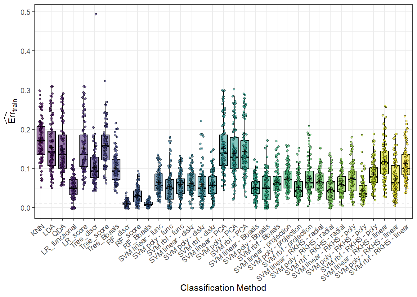
Figure 5.41: Box plots of training errors for 100 simulations for each classification method. Black symbols \(+\) indicate means.
Code
# Set different names for classification methods
methods_names <- c(
'$K$ nearest neighbors',
'Linear discriminant analysis',
'Quadratic discriminant analysis',
'Functional logistic regression',
'Logistic regression with fPCA',
'Decision tree -- discretization',
'Decision tree -- fPCA',
'Decision tree -- basis coefficients',
'Random forest -- discretization',
'Random forest -- fPCA',
'Random forest -- basis coefficients',
'SVM (linear) -- functional',
'SVM (poly) -- functional',
'SVM (radial) -- functional',
'SVM (linear) -- discretization',
'SVM (poly) -- discretization',
'SVM (radial) -- discretization',
'SVM (linear) -- fPCA',
'SVM (poly) -- fPCA',
'SVM (radial) -- fPCA',
'SVM (linear) -- basis coefficients',
'SVM (poly) -- basis coefficients',
'SVM (radial) -- basis coefficients',
'SVM (linear) -- projection',
'SVM (poly) -- projection',
'SVM (radial) -- projection',
'RKHS (radial SVR) $+$ SVM (linear)',
'RKHS (radial SVR) $+$ SVM (poly)',
'RKHS (radial SVR) $+$ SVM (radial)',
'RKHS (poly SVR) $+$ SVM (linear)',
'RKHS (poly SVR) $+$ SVM (poly)',
'RKHS (poly SVR) $+$ SVM (radial)',
'RKHS (linear SVR) $+$ SVM (linear)',
'RKHS (linear SVR) $+$ SVM (poly)',
'RKHS (linear SVR) $+$ SVM (radial)'
)
# Colors for box plots
box_col <- c('#4dd2ff', '#0099cc', '#00ace6', '#00bfff',
'#1ac5ff', rep('#33ccff', 3), rep('#0086b3', 3), rep('#ff3814', 3),
rep('#ff3814', 3), rep('#ff6347', 3), rep('#ff7961', 3),
rep('#ff4d2e', 3), rep('#fa2600', 9))
# box_col <- c('#CA0A0A', '#fa2600', '#fa2600', '#D15804',
# '#D15804', rep('#D3006D', 3), rep('#BE090F', 3), c("#12DEE8", "#4ECBF3", "#127DE8", "#4C3CD3", "#4E65F3", "#4E9EF3", "#081D58") |> rep(each = 3))
# Alpha for box plots
box_alpha <- c(0.9, 0.9, 0.8, 0.9, 0.8, 0.9, 0.8, 0.7, 0.9, 0.8, 0.7,
0.9, 0.8, 0.7, 0.9, 0.8, 0.7, 0.9, 0.8, 0.7, 0.9, 0.8, 0.7, 0.9, 0.8, 0.7,
seq(0.9, 0.6, length = 9)) #- 0.3Code
# Set different names for classification methods
methods_names1 <- c(
'KNN',
'LDA',
'QDA',
'functional LR',
'LR with fPCA',
#'Decision Tree -- Discretization',
#'Decision Tree -- fPCA',
#'Decision Tree -- Basis Coefficients',
'RF -- discretization',
'RF -- fPCA',
'RF -- basis coefficients',
'SVM (linear) -- functional',
'SVM (poly) -- functional',
'SVM (radial) -- functional',
'SVM (linear) -- discretization',
'SVM (poly) -- discretization',
'SVM (radial) -- discretization',
'SVM (linear) -- fPCA',
'SVM (poly) -- fPCA',
'SVM (radial) -- fPCA',
'SVM (linear) -- basis coefficients',
'SVM (poly) -- basis coefficients',
'SVM (radial) -- basis coefficients',
'SVM (linear) -- projection',
'SVM (poly) -- projection',
'SVM (radial) -- projection',
'RKHS (radial SVR) $+$ SVM (linear)',
'RKHS (radial SVR) $+$ SVM (poly)',
'RKHS (radial SVR) $+$ SVM (radial)',
'RKHS (poly SVR) $+$ SVM (linear)',
'RKHS (poly SVR) $+$ SVM (poly)',
'RKHS (poly SVR) $+$ SVM (radial)'#,
#'RKHS (Linear SVR) $+$ SVM (linear)',
#'RKHS (Linear SVR) $+$ SVM (poly)',
#'RKHS (Linear SVR) $+$ SVM (radial)'
)
# Colors for box plots
box_col1 <- c('#4dd2ff', '#00ace6', '#00ace6', '#00bfff', '#00bfff',
rep('#0086b3', 3),
rep('#ff3814', 3), rep('#ff3814', 3), rep('#ff3814', 3), rep('#ff6347', 3), rep('#ff7961', 3),
rep('#ff4d2e', 3), rep('#fa2600', 3))
# Alpha for box plots
box_alpha1 <- c(0.9, 0.9, 0.8, 0.9, 0.8, 0.9, 0.8, 0.7,
rep(c(0.9, 0.8, 0.7), 7)) #- 0.3Code
# for testing data
sub_methods <- methods[c(1:5, 9:32)]
SIMULACE$test |>
pivot_longer(cols = methods, names_to = 'method', values_to = 'Err') |>
mutate(method = factor(method, levels = methods, labels = methods, ordered = TRUE)) |>
as.data.frame() |>
filter(method %in% sub_methods) |>
ggplot(aes(x = method, y = Err, fill = method, colour = method, alpha = method)) +
geom_jitter(position = position_jitter(height = 0, width = 0.15), alpha = 0.6, size = 0.9, pch = 21,
colour = "black") +
geom_boxplot(outlier.colour = "white", outlier.shape = 16, outlier.size = 0,
notch = FALSE, colour = 'black') +
theme_bw() +
labs(x = 'Classification Method',
y = "$\\widehat{\\textnormal{Err}}_{test}$"
# y = expression(widehat(Err)[test])
) +
theme(legend.position = 'none',
axis.text.x = element_text(angle = 45, hjust = 1),
panel.grid.minor = element_blank()) +
stat_summary(fun = "mean", geom = "point", shape = 4,
size = 2, color = "black", alpha = 1) +
scale_x_discrete(labels = methods_names1) +
theme(plot.margin = unit(c(0.1, 0.1, 0.7, 0.5), "cm")) +
scale_fill_manual(values = box_col1) +
scale_alpha_manual(values = box_alpha1) +
coord_cartesian(ylim = c(0, 0.4)) +
geom_hline(yintercept = min(SIMULACE.df$Err.test),
linetype = 'dashed', colour = 'gray20', alpha = 0.8)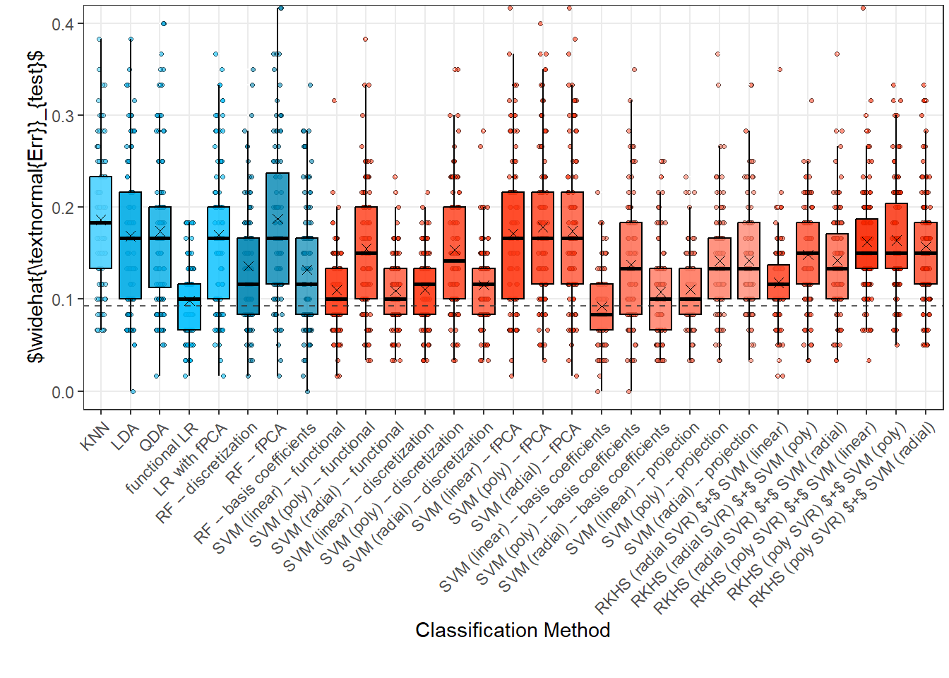
Figure 5.42: Box plots of testing errors for 100 simulations for each classification method. Black symbols \(+\) indicate means.
Code
We would now like to formally test whether some classification methods are better than others based on the previous simulation on these data or if we can consider them equally successful. Since the assumption of normality is not met, we cannot use the classical paired t-test. Instead, we will use its non-parametric alternative—the paired Wilcoxon test. However, we must be cautious with interpretation.
Code
## [1] 0.1256738Code
## [1] 0.003970501Code
## [1] 1.367196e-05We test at an adjusted significance level \(\alpha_{adj} = 0.05 / 3 = 0.0167\).
Finally, let’s take a look at which hyperparameter values were the most common choices.
| Median Hyperparameter Value | |
|---|---|
| KNN_K | 9.0 |
| nharm | 3.0 |
| LR_func_n_basis | 9.5 |
| SVM_d_Linear | 12.0 |
| SVM_d_Poly | 11.0 |
| SVM_d_Radial | 11.0 |
| SVM_RKHS_radial_gamma1 | 100.0 |
| SVM_RKHS_radial_gamma2 | 10.0 |
| SVM_RKHS_radial_gamma3 | 10.0 |
| SVM_RKHS_radial_d1 | 20.0 |
| SVM_RKHS_radial_d2 | 25.0 |
| SVM_RKHS_radial_d3 | 15.0 |
| SVM_RKHS_poly_p1 | 4.0 |
| SVM_RKHS_poly_p2 | 4.0 |
| SVM_RKHS_poly_p3 | 4.0 |
| SVM_RKHS_poly_d1 | 25.0 |
| SVM_RKHS_poly_d2 | 27.5 |
| SVM_RKHS_poly_d3 | 25.0 |
| SVM_RKHS_linear_d1 | 20.0 |
| SVM_RKHS_linear_d2 | 25.0 |
| SVM_RKHS_linear_d3 | 25.0 |
Code
CV_res <- CV_RESULTS |>
  pivot_longer(cols = CV_RESULTS |> colnames(), names_to = 'method', values_to = 'hyperparameter') |>
  mutate(method = factor(method,
                         levels = CV_RESULTS |> colnames(),
                         labels = CV_RESULTS |> colnames(), ordered = TRUE)) |>
  as.data.frame()

CV_res |>
  filter(method %in% c('KNN_K', 'nharm', 'LR_func_n_basis')) |>
  ggplot(aes(x = hyperparameter, #y = after_stat(density),
             fill = method, colour = method)) +
  geom_histogram(binwidth = 1, alpha = 0.6) +
  theme_bw() +
  facet_grid(~method, scales = 'free') +
  labs(x = 'Hyperparameter Values',
       y = 'Absolute Count') +
  theme(legend.position = 'none')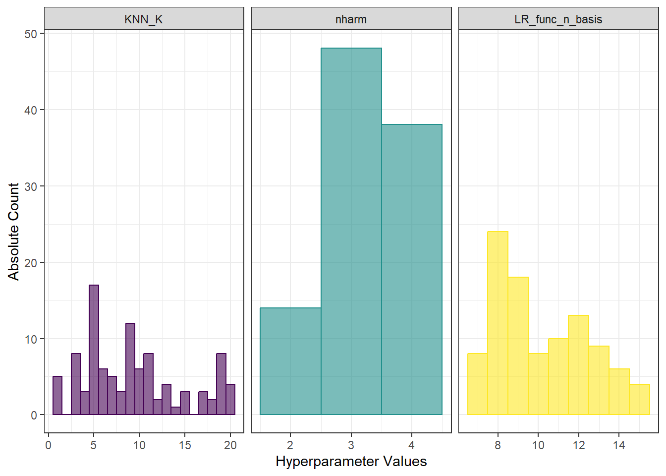
Figure 5.43: Histograms of hyperparameter values for KNN, functional logistic regression, and also a histogram for the number of principal components.
Code
CV_res |>
filter(method %in% c('SVM_d_Linear', 'SVM_d_Poly', 'SVM_d_Radial')) |>
ggplot(aes(x = hyperparameter, #y = after_stat(density),
fill = method, colour = method)) +
geom_histogram(binwidth = 1, alpha = 0.6) +
theme_bw() +
facet_grid(~method, scales = 'free') +
labs(x = 'Hyperparameter Values',
y = 'Absolute Count') +
theme(legend.position = 'none')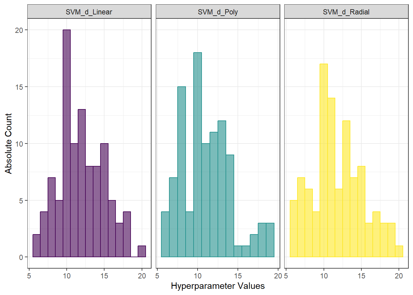
Figure 5.44: Histograms of hyperparameter values for the SVM method with projection onto B-spline basis.
Code
CV_res |>
  filter(method %in% c('SVM_RKHS_radial_gamma1', 'SVM_RKHS_radial_gamma2',
                       'SVM_RKHS_radial_gamma3', 'SVM_RKHS_radial_d1',
                       'SVM_RKHS_radial_d2', 'SVM_RKHS_radial_d3')) |>
  ggplot(aes(x = hyperparameter, #y = after_stat(density),
             fill = method, colour = method)) +
  geom_histogram(bins = 10, alpha = 0.6) +
  theme_bw() +
  facet_wrap(~method, scales = 'free', ncol = 3) +
  labs(x = 'Hyperparameter Values',
       y = 'Absolute Count') +
  theme(legend.position = 'none')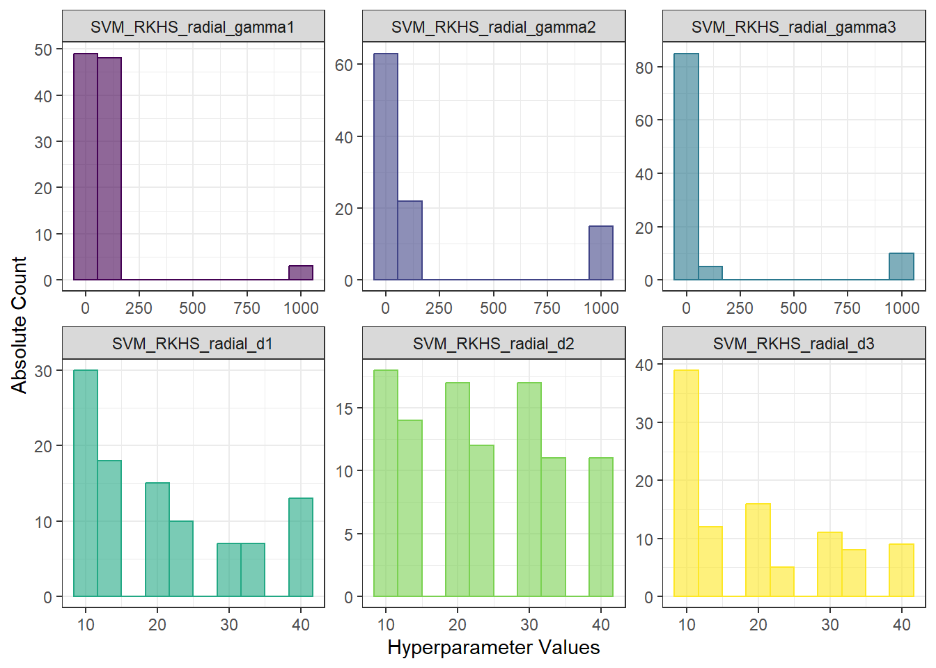
Figure 5.45: Histograms of hyperparameter values for the RKHS + SVM with radial kernel method.
Code
CV_res |>
  filter(method %in% c('SVM_RKHS_poly_p1', 'SVM_RKHS_poly_p2',
                       'SVM_RKHS_poly_p3', 'SVM_RKHS_poly_d1',
                       'SVM_RKHS_poly_d2', 'SVM_RKHS_poly_d3')) |>
  ggplot(aes(x = hyperparameter, #y = after_stat(density),
             fill = method, colour = method)) +
  geom_histogram(binwidth = 1, alpha = 0.6) +
  theme_bw() +
  facet_wrap(~method, scales = 'free', ncol = 3) +
  labs(x = 'Hyperparameter Values',
       y = 'Absolute Count') +
  theme(legend.position = 'none')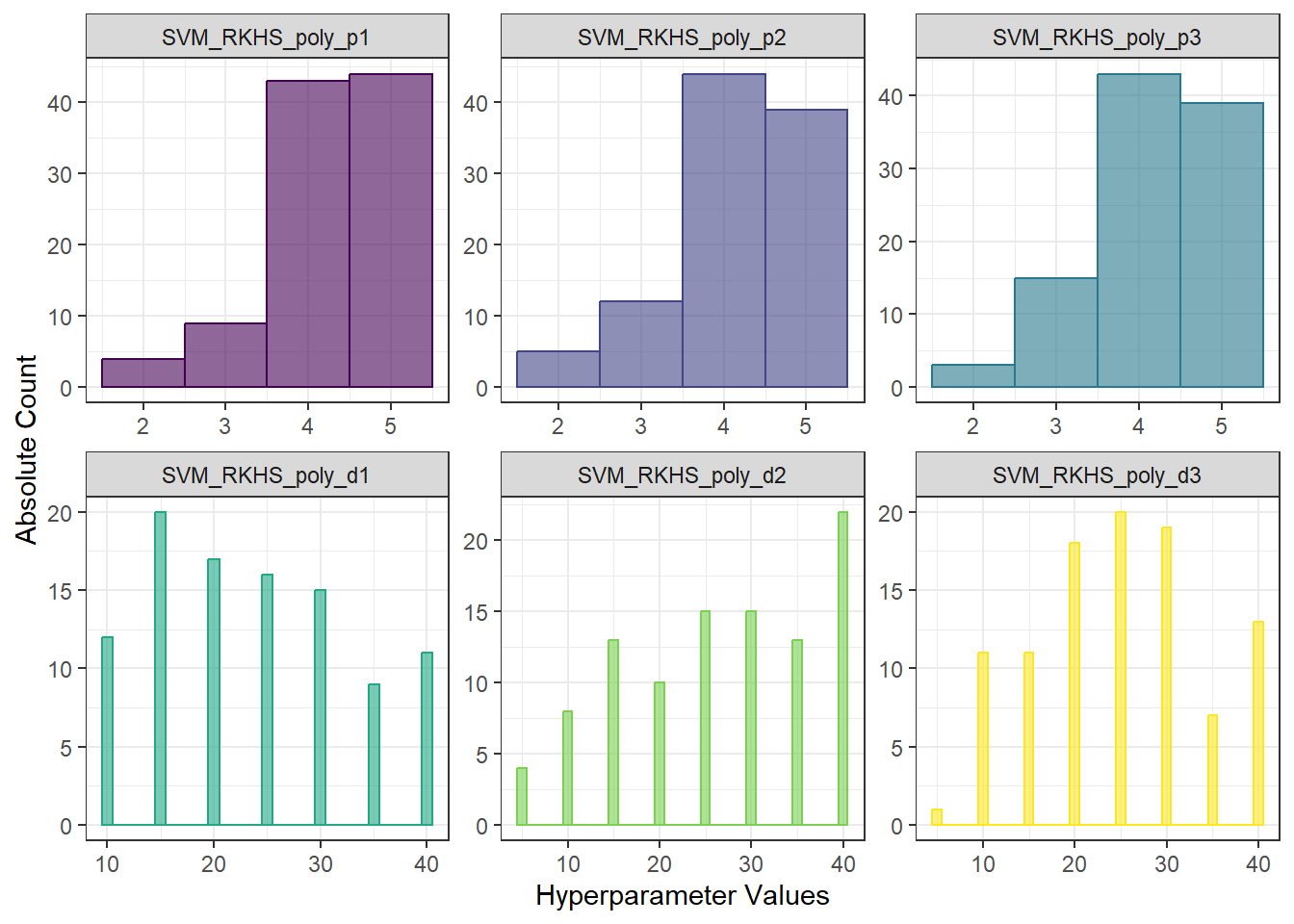
Figure 5.46: Histograms of hyperparameter values for the RKHS + SVM with polynomial kernel method.
Code
CV_res |>
  filter(method %in% c('SVM_RKHS_linear_d1',
                       'SVM_RKHS_linear_d2', 'SVM_RKHS_linear_d3')) |>
  ggplot(aes(x = hyperparameter, #y = after_stat(density),
             fill = method, colour = method)) +
  geom_histogram(binwidth = 5, alpha = 0.6) +
  theme_bw() +
  facet_wrap(~method, scales = 'free', ncol = 3) +
  labs(x = 'Hyperparameter Values',
       y = 'Absolute Count') +
  theme(legend.position = 'none')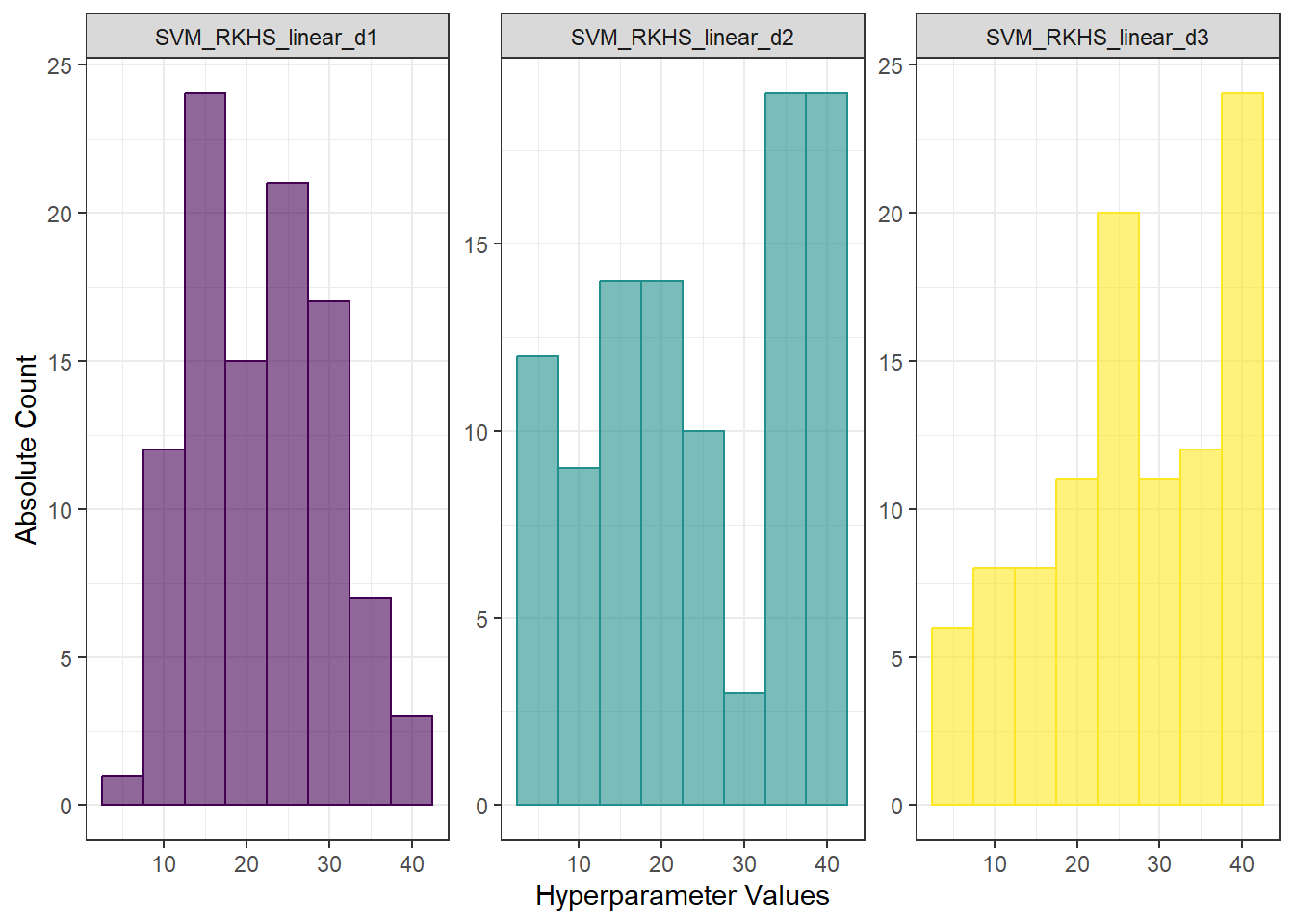
Figure 5.47: Histograms of hyperparameter values for the RKHS + SVM with linear kernel method.
Let’s finally compare the best classifiers from each derivative, namely the linear SVM applied to the coefficients of orthogonal projection onto the B-spline function system for the non-derivative data (error rate of \(9.55\,\%\)) and applied to the basis coefficients for the first (error rate of \(9.58\,\%\)) and second (error rate of \(9.32\,\%\)) derivatives.
Since in all three simulation studies we set the pseudorandom number generator to the same value, the generated discrete vectors \(\boldsymbol y_i\) and their distribution into sets \(\mathcal T_1\) and \(\mathcal T_2\) are identical for the given repetition out of the total \(N=100\). Therefore, to compare the medians of the test error rates of the most successful methods, we will again use the Wilcoxon paired test.
Code
Let’s check that we have loaded the correct data.
## [1] 0.09316667## [1] 0.1## [1] 0.0925Finally, we will conduct formal tests.
Code
##
## Wilcoxon signed rank test with continuity correction
##
## data: data_0der$test$`SVM linear - projection` and data_1der$test$`SVM linear - Bbasis`
## V = 1939, p-value = 0.2058
## alternative hypothesis: true location shift is not equal to 0Code
##
## Wilcoxon signed rank test with continuity correction
##
## data: data_0der$test$`SVM linear - projection` and data_2der$test$`SVM linear - Bbasis`
## V = 1866.5, p-value = 0.988
## alternative hypothesis: true location shift is not equal to 0Code
##
## Wilcoxon signed rank test with continuity correction
##
## data: data_1der$test$`SVM linear - Bbasis` and data_2der$test$`SVM linear - Bbasis`
## V = 2424, p-value = 0.1902
## alternative hypothesis: true location shift is not equal to 0We see that all three \(p\)-values are significantly above the significance level of 0.05 (and even after adjustment), so we can conclude that the classification power of these methods is comparable.