Chapter 4 Dependency on Discretization

In this section, we will focus on the dependence of the results from the previous section 1 on the value of $p$, which defines the length of the equidistant sequence of points used for discretizing the observed functional objects. We are interested in how the error rates of individual classification methods change as we refine the interval division, that is, as the dimension of the discretized vectors increases.

Our assumption is that the support vector method applied to discretized data should yield lower error rates as $p$ increases, since we better approximate integrals and thus the values of kernel functions for functional analogs. Conversely, we would expect decision trees and random forests to stagnate beyond a certain number of $p$.

Since we are discussing the discretization of the interval, this chapter will focus solely on methods that work with discretized data—namely:

Decision Tree,
Random Forest,
SVM Method.

In addition to average test error rates, we are also interested in the computational cost of each method as $p$ increases, since minimum error rate is not the only criterion for using a given classification method in practice. Computational complexity and the associated time demands play a relatively important role as well.

This chapter consists of two parts. In the first Section 4.3, we will choose a fixed number of $p=101$ discretized values and examine the individual methods, their error rates, and their time demands. Subsequently, in Section 4.4, we will define a sequence of $p$ values and repeat the entire process several times for each value so that we can establish average results for that value. Finally, we will plot the dependence of error rates and computational demands on the value of $p$.

4.1 Simulation of Functional Data

First, we will simulate functions that we will later classify. For simplicity, we will consider two classification classes. To simulate, we will:

choose appropriate functions,
generate points from the chosen interval that contain, for example, Gaussian noise,
smooth the resulting discrete points into the form of a functional object using a suitable basis system.

This process will yield functional objects along with the value of the categorical variable $Y$, which distinguishes class membership.

Code

# Load necessary packages

library(fda)
library(ggplot2)
library(dplyr)
library(tidyr)
library(ddalpha)
library(polynom)

set.seed(42)

Let’s consider two classification classes, $Y \in \{0, 1\}$, with the same number of generated functions n for each class. First, we will define two functions, each for one class, over the interval $I = [0, 6]$.

Now we will create functions using interpolation polynomials. First, we define the points that our curve should pass through and then fit an interpolation polynomial through them, which we will use to generate curves for classification.

Code

# Defining points for class 0
x.0 <- c(0.00, 0.65, 0.94, 1.42, 2.26, 2.84, 3.73, 4.50, 5.43, 6.00)
y.0 <- c(0, 0.25, 0.86, 1.49, 1.1, 0.15, -0.11, -0.36, 0.23, 0)

# Defining points for class 1
x.1 <- c(0.00, 0.51, 0.91, 1.25, 1.51, 2.14, 2.43, 2.96, 3.70, 4.60,
         5.25, 5.67, 6.00)
y.1 <- c(0.1, 0.4, 0.71, 1.08, 1.47, 1.39, 0.81, 0.05, -0.1, -0.4,
         0.3, 0.37, 0)

Code

# Plot points
dat_points <- data.frame(x = c(x.0, x.1),
                         y = c(y.0, y.1),
                         Class = rep(c('Y = 0', 'Y = 1'), 
                                     c(length(x.0), length(x.1))))

ggplot(dat_points, aes(x = x, y = y, colour = Class)) + 
  geom_point(size=1.5) + 
  theme_bw() + 
  labs(colour = 'Classification\n      Class')

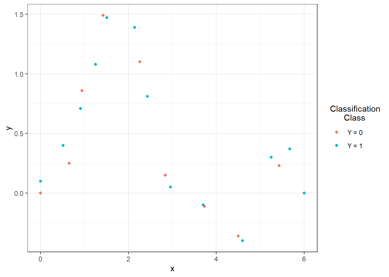
Figure 1.1: Points defining the interpolation polynomials.

To calculate the interpolation polynomials, we will use the poly.calc() function from the polynom library. We will then define functions poly.0() and poly.1() that will compute the polynomial values at a given point in the interval. To create these, we will use the predict() function, where we input the corresponding polynomial and the point at which we want to evaluate the polynomial.

Code

# Calculate polynomials
polynom.0 <- poly.calc(x.0, y.0)
polynom.1 <- poly.calc(x.1, y.1)

Code

poly.0 <- function(x) return(predict(polynom.0, x))
poly.1 <- function(x) return(predict(polynom.1, x))

Code

# Plot polynomials
xx <- seq(min(x.0), max(x.0), length = 501)
yy.0 <- poly.0(xx)
yy.1 <- poly.1(xx)

dat_poly_plot <- data.frame(x = c(xx, xx),
                            y = c(yy.0, yy.1),
                            Class = rep(c('Y = 0', 'Y = 1'), 
                                        c(length(xx), length(xx))))

ggplot(dat_points, aes(x = x, y = y, colour = Class)) + 
  geom_point(size=1.5) + 
  theme_bw() + 
  geom_line(data = dat_poly_plot,
            aes(x = x, y = y, colour = Class),
            linewidth = 0.8) + 
  labs(colour = 'Classification\n      Class')

Figure 1.2: Representation of two functions over the interval $I = [0, 6]$, from which we generate observations from classes 0 and 1.

Code

# Generating functions for Y = 0 and Y = 1
funkce_0 <- poly.0
funkce_1 <- poly.1

Now we will create a function to generate random functions with added noise (or points on a predefined grid) from the chosen generating function. The argument t indicates the vector of values at which we want to evaluate the functions, fun denotes the generating function, n is the number of functions, and sigma is the standard deviation of the normal distribution $\text{N}(\mu, \sigma^2)$, from which we randomly generate Gaussian white noise with $\mu = 0$. To demonstrate the advantage of using methods that work with functional data, we will also add a random term to each simulated observation, which will serve as a vertical shift for the entire function (parameter sigma_shift). This shift will be generated from a normal distribution with the parameter $\sigma^2 = 4$.

Code

generate_values <- function(t, fun, n, sigma, sigma_shift = 0) {
  # Arguments:
  # t ... vector of values, where the function will be evaluated
  # fun ... generating function of t 
  # n ... the number of generated functions / objects
  # sigma ... standard deviation of normal distribution to add noise to data
  # sigma_shift ... parameter of normal distribution for generating shift
  
  # Value:
  # X ... matrix of dimension length(t) times n with generated values of one 
  # function in a column 
  
  X <- matrix(rep(t, times = n), ncol = n, nrow = length(t), byrow = FALSE)
  noise <- matrix(rnorm(n * length(t), mean = 0, sd = sigma),
                  ncol = n, nrow = length(t), byrow = FALSE)
  shift <- matrix(rep(rnorm(n, 0, sigma_shift), each = length(t)),
                  ncol = n, nrow = length(t))
  return(fun(X) + noise + shift)
}

Now we can generate the functions. In each of the two classes, we will consider 100 observations, thus n = 100.

Code

# Number of generated observations for each class
n <- 100
# Vector of time points equidistant on the interval [0, 6]
t <- seq(0, 6, length = 51)

# For Y = 0
X0 <- generate_values(t, funkce_0, n, 1, 2)
# For Y = 1
X1 <- generate_values(t, funkce_1, n, 1, 2)

We will plot the generated (not yet smoothed) functions in color according to their class (only the first 10 observations from each class for clarity).

Code

n_curves_plot <- 10 # Number of curves to plot from each group

DF0 <- cbind(t, X0[, 1:n_curves_plot]) |> 
  as.data.frame() |> 
  reshape(varying = 2:(n_curves_plot + 1), direction = 'long', sep = '') |> 
  subset(select = -id) |> 
  mutate(
  time = time - 1,
  group = 0
  )

DF1 <- cbind(t, X1[, 1:n_curves_plot]) |> 
  as.data.frame() |> 
  reshape(varying = 2:(n_curves_plot + 1), direction = 'long', sep = '') |> 
  subset(select = -id) |> 
  mutate(
  time = time - 1,
  group = 1
  )

DF <- rbind(DF0, DF1) |>
  mutate(group = factor(group))

DF |> ggplot(aes(x = t, y = V, group = interaction(time, group), 
                 colour = group)) + 
  geom_line(linewidth = 0.5) +
  theme_bw() +
  labs(x = expression(x[1]),
       y = expression(x[2]),
       colour = 'Classification\n      Class') +
  scale_colour_discrete(labels=c('Y = 0', 'Y = 1'))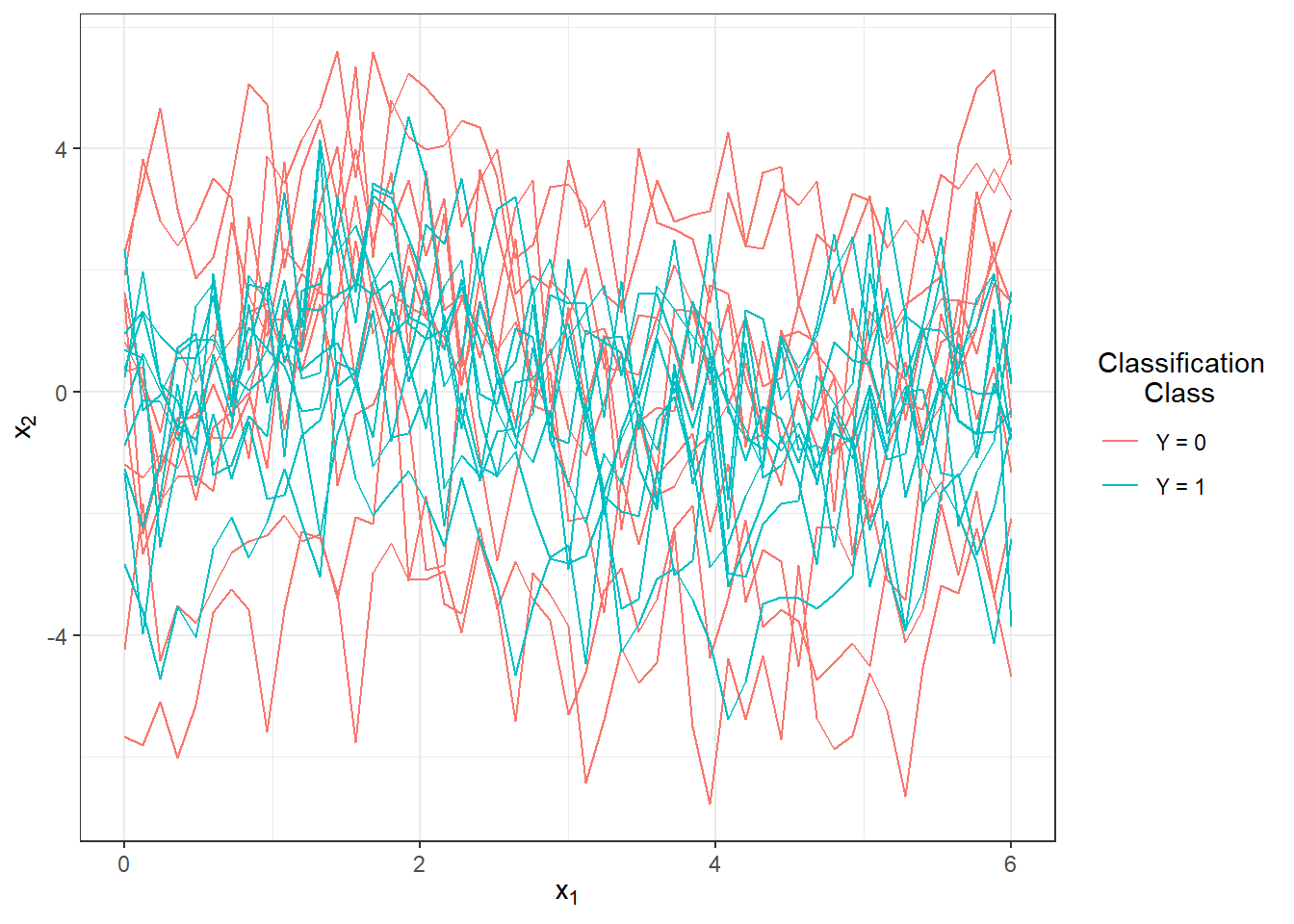

Figure 1.3: The first 10 generated observations from each of the two classification classes. The observed data are not smoothed.

4.2 Smoothing the Observed Curves

Now we will convert the observed discrete values (vectors of values) into functional objects, which we will subsequently work with. We will again use a B-spline basis for smoothing.

We will take the entire vector t as the knots, and since we will generally consider cubic splines, we will choose (the default choice in R) norder = 4. We will penalize the second derivative of the functions.

Code

rangeval <- range(t)
breaks <- t
norder <- 4

bbasis <- create.bspline.basis(rangeval = rangeval, 
                               norder = norder, 
                               breaks = breaks)

curv.Lfd <- int2Lfd(2) # penalize the 2nd derivative

We will find a suitable value for the smoothing parameter $\lambda > 0$ using $GCV(\lambda)$, i.e., using generalized cross-validation. We will consider the value of $\lambda$ to be the same for both classification groups because we would not know in advance which value of $to choose if a different choice were made for each class.

Code

# Combine observations into a single matrix
XX <- cbind(X0, X1)

lambda.vect <- 10^seq(from = -2, to = 1, length.out = 50) # vector of lambdas
gcv <- rep(NA, length = length(lambda.vect)) # empty vector for storing GCV

for(index in 1:length(lambda.vect)) {
  curv.Fdpar <- fdPar(bbasis, curv.Lfd, lambda.vect[index])
  BSmooth <- smooth.basis(t, XX, curv.Fdpar) # smoothing
  gcv[index] <- mean(BSmooth$gcv) # average over all observed curves
}

GCV <- data.frame(
  lambda = round(log10(lambda.vect), 3),
  GCV = gcv
)

# Find the minimum value
lambda.opt <- lambda.vect[which.min(gcv)]

For better visualization, we will plot the progression of $GCV(\lambda)$.

Code

GCV |> ggplot(aes(x = lambda, y = GCV)) + 
  geom_line(linetype = 'solid', linewidth = 0.6) + 
  geom_point(size = 1.5) + 
  theme_bw() + 
  labs(x = bquote(paste(log[10](lambda), ' ;   ', 
                        lambda[optimal] == .(round(lambda.opt, 4)))),
       y = expression(GCV(lambda))) + 
  geom_point(aes(x = log10(lambda.opt), y = min(gcv)), colour = 'red', size = 2.5)

## Warning in geom_point(aes(x = log10(lambda.opt), y = min(gcv)), colour = "red", : All aesthetics have length 1, but the data has 50 rows.
## ℹ Please consider using `annotate()` or provide this layer with data containing
##   a single row.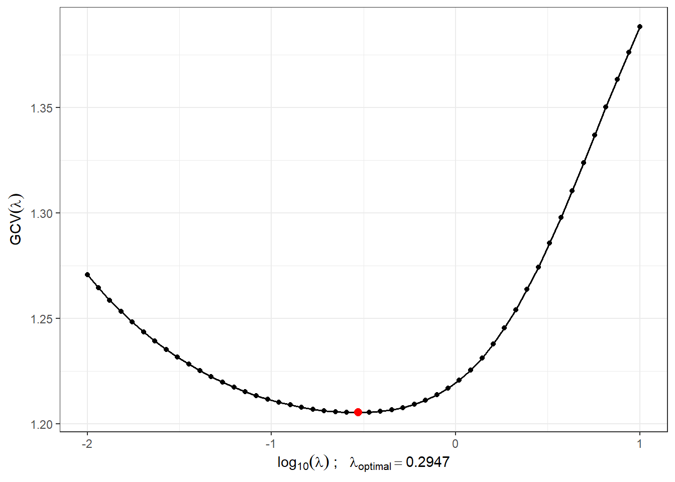

$The progression of $GCV(\lambda)$ for the chosen vector $\boldsymbol\lambda$. The x-axis values are plotted on a logarithmic scale. The optimal value of the smoothing parameter $\lambda_{optimal}$ is indicated in red.$

Figure 1.4: The progression of $GCV(\lambda)$ for the chosen vector $\boldsymbol\lambda$. The x-axis values are plotted on a logarithmic scale. The optimal value of the smoothing parameter $\lambda_{optimal}$ is indicated in red.

With this optimal choice of the smoothing parameter $\lambda$, we will now smooth all functions and again graphically display the first 10 observed curves from each classification class.

Code

curv.fdPar <- fdPar(bbasis, curv.Lfd, lambda.opt)
BSmooth <- smooth.basis(t, XX, curv.fdPar)
XXfd <- BSmooth$fd

fdobjSmootheval <- eval.fd(fdobj = XXfd, evalarg = t)
DF$Vsmooth <- c(fdobjSmootheval[, c(1 : n_curves_plot, 
                                    (n + 1) : (n + n_curves_plot))])

DF |> ggplot(aes(x = t, y = Vsmooth, group = interaction(time, group), 
                 colour = group)) + 
  geom_line(linewidth = 0.75) +
  theme_bw() +
  labs(x = expression(x[1]),
       y = expression(x[2]),
       colour = 'Classification\n      Class') +
  scale_colour_discrete(labels=c('Y = 0', 'Y = 1'))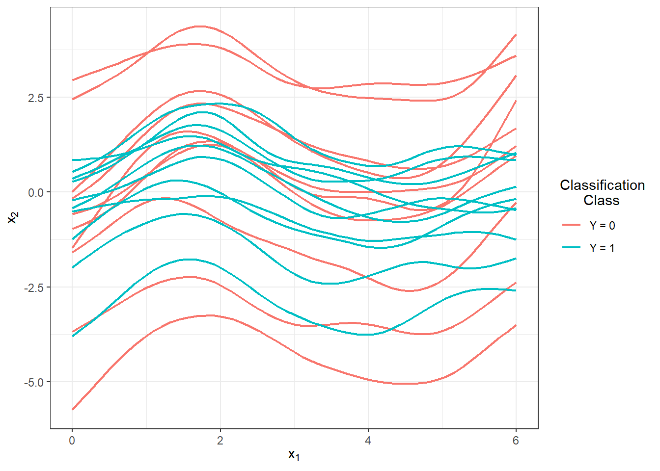

Figure 1.5: The first 10 smoothed curves from each classification class.

Let’s visualize all the smoothed observed curves, highlighting them by their classification class, along with the average for each class.

Code

DFsmooth <- data.frame(
  t = rep(t, 2 * n),
  time = rep(rep(1:n, each = length(t)), 2),
  Smooth = c(fdobjSmootheval),
  Mean = c(rep(apply(fdobjSmootheval[ , 1 : n], 1, mean), n),
            rep(apply(fdobjSmootheval[ , (n + 1) : (2 * n)], 1, mean), n)),
  group = factor(rep(c(0, 1), each = n * length(t)))
)

DFmean <- data.frame(
  t = rep(t, 2),
  Mean = c(apply(fdobjSmootheval[ , 1 : n], 1, mean), 
            apply(fdobjSmootheval[ , (n + 1) : (2 * n)], 1, mean)),
  group = factor(rep(c(0, 1), each = length(t)))
)

DFsmooth |> ggplot(aes(x = t, y = Smooth, group = interaction(time, group), 
                 colour = group)) + 
  geom_line(linewidth = 0.25, alpha = 0.5) +
  theme_bw() +
  labs(x = expression(x[1]),
       y = expression(x[2]),
       colour = 'Classification\n      Class') +
  scale_colour_discrete(labels = c('Y = 0', 'Y = 1')) + 
  geom_line(aes(x = t, y = Mean, colour = group), 
            linewidth = 1.2, linetype = 'solid') + 
  scale_x_continuous(expand = c(0.01, 0.01)) + 
  scale_y_continuous(expand = c(0.01, 0.01)) # limits = c(-1, 2)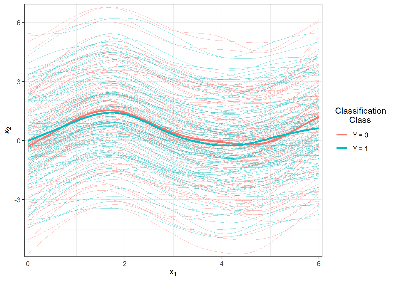

Figure 1.6: Plot of all smoothed observed curves, colored by classification class. The thick line represents the average for each class.

Code

DFsmooth <- data.frame(
  t = rep(t, 2 * n),
  time = rep(rep(1:n, each = length(t)), 2),
  Smooth = c(fdobjSmootheval),
  Mean = c(rep(apply(fdobjSmootheval[ , 1 : n], 1, mean), n),
            rep(apply(fdobjSmootheval[ , (n + 1) : (2 * n)], 1, mean), n)),
  group = factor(rep(c(0, 1), each = n * length(t)))
)

DFmean <- data.frame(
  t = rep(t, 2),
  Mean = c(apply(fdobjSmootheval[ , 1 : n], 1, mean), 
            apply(fdobjSmootheval[ , (n + 1) : (2 * n)], 1, mean)),
  group = factor(rep(c(0, 1), each = length(t)))
)

DFsmooth |> ggplot(aes(x = t, y = Smooth, group = interaction(time, group), 
                 colour = group)) + 
  geom_line(linewidth = 0.25, alpha = 0.5) +
  theme_bw() +
  labs(x = expression(x[1]),
       y = expression(x[2]),
       colour = 'Classification\n      Class') +
  scale_colour_discrete(labels = c('Y = 0', 'Y = 1')) + 
  geom_line(aes(x = t, y = Mean, colour = group), 
            linewidth = 1.2, linetype = 'solid') + 
  scale_x_continuous(expand = c(0.01, 0.01)) + 
  scale_y_continuous(expand = c(0.01, 0.01), limits = c(-1, 2))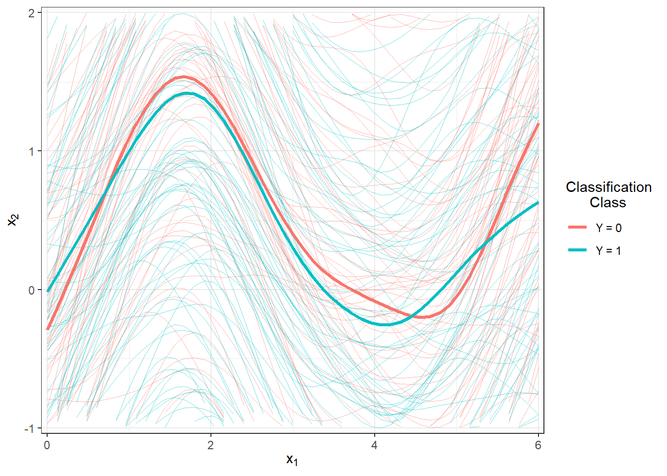

Plot of all smoothed observed curves, colored by classification class. The thick line represents the average for each class. Close-up view.

Figure 1.7: Plot of all smoothed observed curves, colored by classification class. The thick line represents the average for each class. Close-up view.

Here’s the continuation of your text, including the code for classification with decision trees.

4.3 Classification of Curves

First, we will load the necessary libraries for classification.

Code

library(caTools) # for splitting into test and training sets
library(caret) # for k-fold CV
library(fda.usc) # for KNN, fLR
library(MASS) # for LDA
library(fdapace)
library(pracma)
library(refund) # for LR on scores
library(nnet) # for LR on scores
library(caret)
library(rpart) # decision trees
library(rattle) # graphics
library(e1071)
library(randomForest) # random forest

To compare the individual classifiers, we will split the generated observations into two parts in a ratio of 70:30, designated as training and test (validation) sets. The training set will be used for constructing the classifier, while the test set will be used for calculating classification errors and potentially other model characteristics. We can then compare the resulting classifiers based on these computed characteristics regarding their classification success.

Code

# splitting into test and training sets
split <- sample.split(XXfd$fdnames$reps, SplitRatio = 0.7)

Y <- rep(c(0, 1), each = n)

X.train <- subset(XXfd, split == TRUE)
X.test <- subset(XXfd, split == FALSE)

Y.train <- subset(Y, split == TRUE)
Y.test <- subset(Y, split == FALSE)

Next, we will examine the representation of individual groups in the test and training data.

4.3.1 Decision Trees

Decision trees are a popular tool for classification; however, similar to some previous methods, they are not directly designed for functional data. Nevertheless, there are ways to convert functional objects into multidimensional ones and then apply decision tree algorithms to them. We can consider the following approaches:

An algorithm constructed on basis coefficients,
Using scores of principal components,
Discretizing the interval and evaluating the function only at some finite grid points.

We will, of course, choose the last option. First, we need to define points from the interval $I = [0, 6]$ at which we will evaluate the functions. Next, we will create an object where the rows represent individual (discretized) functions and the columns represent time. Finally, we will append a column $Y$ with information about classification class membership and repeat the same for the test data.

Code

# sequence of points where we evaluate the functions
p <- 101
t.seq <- seq(0, 6, length = p)

grid.data <- eval.fd(fdobj = X.train, evalarg = t.seq)
grid.data <- as.data.frame(t(grid.data)) # transpose for functions in rows
grid.data$Y <- Y.train |> factor()

grid.data.test <- eval.fd(fdobj = X.test, evalarg = t.seq)
grid.data.test <- as.data.frame(t(grid.data.test))
grid.data.test$Y <- Y.test |> factor()

Now we can construct a decision tree, using all the times from the vector t.seq as predictors. This classification is not sensitive to multicollinearity, so we do not need to concern ourselves with it. We will choose accuracy as the metric.

Code

# constructing the model
start_time <- Sys.time()
clf.tree <- train(Y ~ ., data = grid.data, 
                 method = "rpart", 
                 trControl = trainControl(method = "CV", number = 10),
                 metric = "Accuracy")
end_time <- Sys.time()

# accuracy on training data
predictions.train <- predict(clf.tree, newdata = grid.data)
accuracy.train <- table(Y.train, predictions.train) |>
  prop.table() |> diag() |> sum()

# accuracy on test data
predictions.test <- predict(clf.tree, newdata = grid.data.test)
accuracy.test <- table(Y.test, predictions.test) |>
  prop.table() |> diag() |> sum()

The error rate of the classifier on the test data is therefore 46.67 %, and on the training data, it is 33.57 %. We will calculate the time taken as follows.

Code

duration <- end_time - start_time
duration |> print()

## Time difference of 0.718204 secs

We can graphically visualize the decision tree using the fancyRpartPlot() function. We will set the colors of the nodes to reflect the previous color differentiation. This will be an unpruned tree.

Code

colnames(grid.data) <- c(paste0('time:', t.seq), 'Y')
fancyRpartPlot(rpart(Y ~ ., data = grid.data, method = "class"),
               sub = '', palettes = c('Reds', 'Blues'))

Graphical representation of the unpruned decision tree. Nodes belonging to classification class 1 are shown in shades of blue, and those belonging to class 0 are in shades of red.

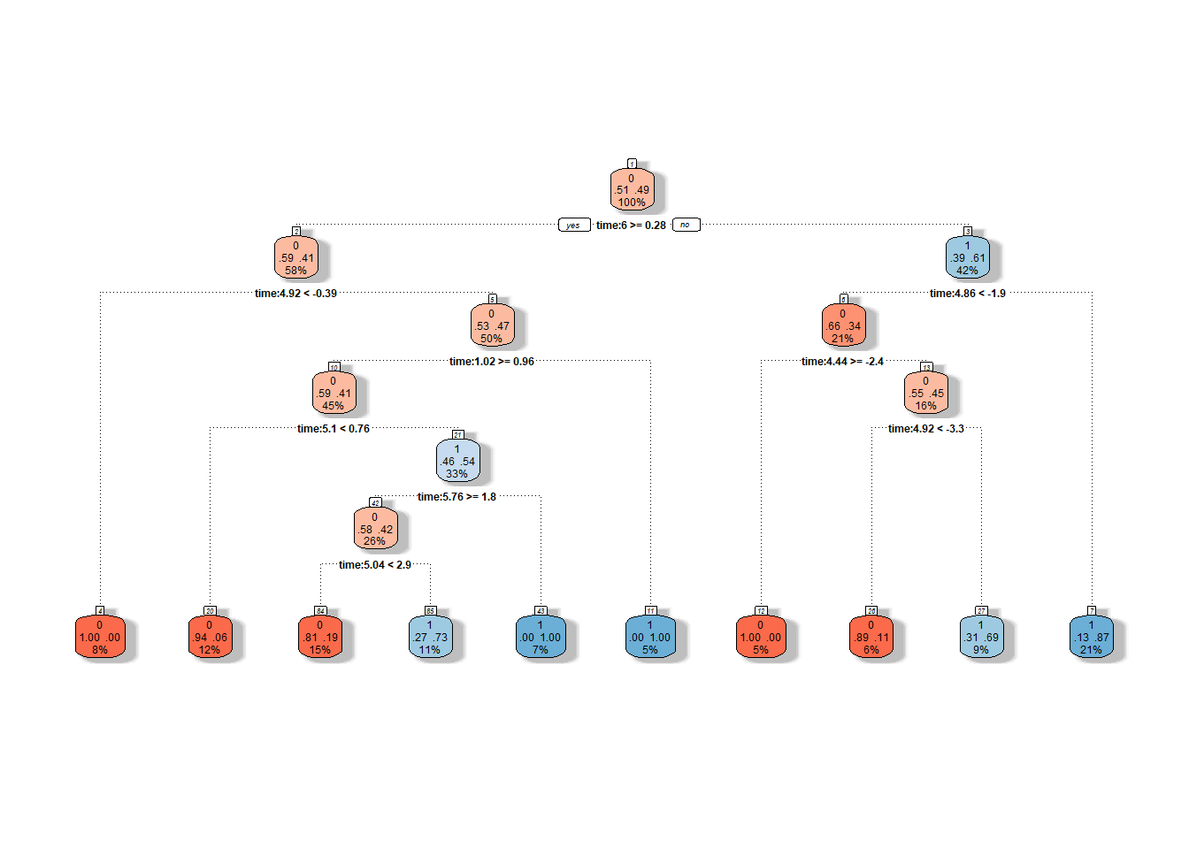
Figure 1.8: Graphical representation of the unpruned decision tree. Nodes belonging to classification class 1 are shown in shades of blue, and those belonging to class 0 are in shades of red.

We can also plot the final pruned decision tree.

Code

rpart.plot::rpart.plot(clf.tree$finalModel, # final model ... pruned tree
                       extra = 104, # display required information
                       box.palette = c('Reds', 'Blues'),
                       branch.lty = 3, # dotted branch lines
                       shadow.col = 0, # shadows under the node boxes
                       nn = FALSE, 
                       under = FALSE, 
                       digits = 2)

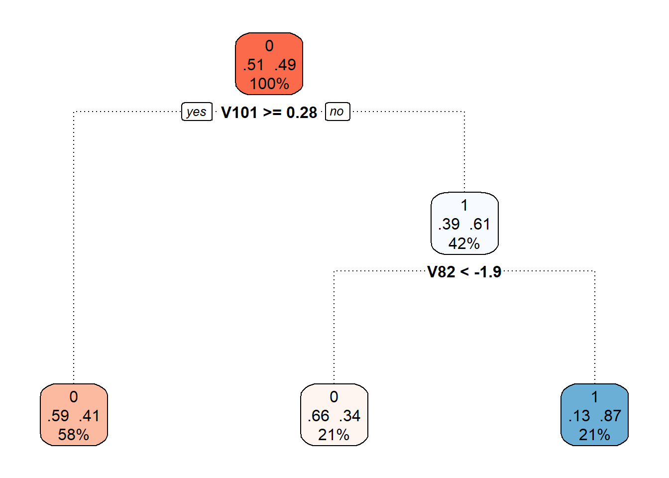
Figure 2.3: Final pruned decision tree.

Finally, let’s add the training and test error rates to the summary table.

Code

RESULTS <- data.frame(model = 'Tree - discr.', 
                  Err.train = 1 - accuracy.train,
                  Err.test = 1 - accuracy.test,
                  Duration = as.numeric(duration))

4.3.2 Random Forests

The classifier constructed using the random forests method consists of building several individual decision trees, which are subsequently combined to create a common classifier (through a collective “vote”).

As with decision trees, we have several options regarding what data (finite-dimensional) to use for constructing the model. We will again consider discretization of the interval. In this case, we utilize the evaluation of functions on a given grid of points in the interval $I = [0, 6]$.

Code

# model construction
start_time <- Sys.time()
clf.RF <- randomForest(Y ~ ., data = grid.data, 
                       ntree = 500, # number of trees
                       importance = F,
                       nodesize = 1)
end_time <- Sys.time()

# accuracy on training data
predictions.train <- predict(clf.RF, newdata = grid.data)
presnost.train <- table(Y.train, predictions.train) |>
  prop.table() |> diag() |> sum()
  
# accuracy on test data
predictions.test <- predict(clf.RF, newdata = grid.data.test)
presnost.test <- table(Y.test, predictions.test) |>
  prop.table() |> diag() |> sum()

The error rate of the random forest on the training data is therefore 0 % and on the test data 40 %. We will calculate the time complexity as follows.

Code

duration <- end_time - start_time
duration |> print()

## Time difference of 0.302609 secs

Code

Res <- data.frame(model = 'RForest - discr', 
                  Err.train = 1 - presnost.train,
                  Err.test = 1 - presnost.test,
                  Duration = as.numeric(duration))

RESULTS <- rbind(RESULTS, Res)

4.3.3 Support Vector Machines

Now let’s look at classifying our simulated curves using the Support Vector Machines (SVM) method. The advantage of this classification method is its computational efficiency, as it uses only a few (often very few) observations to define the boundary curve between classes.

In the case of functional data, we have several options for applying the SVM method. The simplest variant is to use this classification method directly on the discretized function. We will start by applying the support vector method directly to the discretized data (evaluation of the function on a given grid of points in the interval $I = [0, 6]$), considering all three aforementioned kernel functions. First, however, we will normalize the data.

Code

# set norm equal to one
norms <- c()
for (i in 1:dim(XXfd$coefs)[2]) {
  norms <- c(norms, as.numeric(1 / norm.fd(XXfd[i])))
  }
XXfd_norm <- XXfd 
XXfd_norm$coefs <- XXfd_norm$coefs * matrix(norms, 
                                            ncol = dim(XXfd$coefs)[2],
                                            nrow = dim(XXfd$coefs)[1],
                                            byrow = T)

# split into test and training parts
X.train_norm <- subset(XXfd_norm, split == TRUE)
X.test_norm <- subset(XXfd_norm, split == FALSE)

Y.train_norm <- subset(Y, split == TRUE)
Y.test_norm <- subset(Y, split == FALSE)

grid.data <- eval.fd(fdobj = X.train_norm, evalarg = t.seq)
grid.data <- as.data.frame(t(grid.data)) 
grid.data$Y <- Y.train_norm |> factor()

grid.data.test <- eval.fd(fdobj = X.test_norm, evalarg = t.seq)
grid.data.test <- as.data.frame(t(grid.data.test))
grid.data.test$Y <- Y.test_norm |> factor()

Code

# model construction
start_time <- Sys.time()
clf.SVM.l <- svm(Y ~ ., data = grid.data,
                 type = 'C-classification',
                 scale = TRUE,
                 cost = 100,
                 kernel = 'linear')
end_time <- Sys.time()

duration.l <- end_time - start_time

start_time <- Sys.time()
clf.SVM.p <- svm(Y ~ ., data = grid.data,
                 type = 'C-classification',
                 scale = TRUE,
                 coef0 = 1,
                 cost = 100,
                 kernel = 'polynomial')
end_time <- Sys.time()

duration.p <- end_time - start_time

start_time <- Sys.time()
clf.SVM.r <- svm(Y ~ ., data = grid.data,
                 type = 'C-classification',
                 scale = TRUE,
                 cost = 100000,
                 gamma = 0.0001,
                 kernel = 'radial')
end_time <- Sys.time()

duration.r <- end_time - start_time

# accuracy on training data
predictions.train.l <- predict(clf.SVM.l, newdata = grid.data)
presnost.train.l <- table(Y.train, predictions.train.l) |>
  prop.table() |> diag() |> sum()

predictions.train.p <- predict(clf.SVM.p, newdata = grid.data)
presnost.train.p <- table(Y.train, predictions.train.p) |>
  prop.table() |> diag() |> sum()

predictions.train.r <- predict(clf.SVM.r, newdata = grid.data)
presnost.train.r <- table(Y.train, predictions.train.r) |>
  prop.table() |> diag() |> sum()

# accuracy on test data
predictions.test.l <- predict(clf.SVM.l, newdata = grid.data.test)
presnost.test.l <- table(Y.test, predictions.test.l) |>
  prop.table() |> diag() |> sum()

predictions.test.p <- predict(clf.SVM.p, newdata = grid.data.test)
presnost.test.p <- table(Y.test, predictions.test.p) |>
  prop.table() |> diag() |> sum()

predictions.test.r <- predict(clf.SVM.r, newdata = grid.data.test)
presnost.test.r <- table(Y.test, predictions.test.r) |>
  prop.table() |> diag() |> sum()

The error rate of the SVM method on the training data is therefore 5.71 % for the linear kernel, 2.14 % for the polynomial kernel, and 3.57 % for the Gaussian kernel. On the test data, the error rate of the method is 16.67 % for the linear kernel, 16.67 % for the polynomial kernel, and 13.33 % for the radial kernel. We will calculate the time complexity as follows.

Code

print('Linear kernel:', quote = F)

## [1] Linear kernel:

Code

duration.l |> print()

## Time difference of 0.04756021 secs

Code

print('Polynomial kernel:', quote = F)

## [1] Polynomial kernel:

Code

duration.p |> print()

## Time difference of 0.03182602 secs

Code

print('Radial kernel:', quote = F)

## [1] Radial kernel:

Code

duration.r |> print()

## Time difference of 0.06402302 secs

Code

Res <- data.frame(model = c('SVM linear - discr', 
                            'SVM poly - discr', 
                            'SVM rbf - discr'), 
                  Err.train = 1 - c(presnost.train.l, presnost.train.p, presnost.train.r),
                  Err.test = 1 - c(presnost.test.l, presnost.test.p, presnost.test.r),
                  Duration = c(as.numeric(duration.l), 
                               as.numeric(duration.p), as.numeric(duration.r)))

RESULTS <- rbind(RESULTS, Res)

4.3.4 Results Table

Table 4.1: Summary of results of the methods used on simulated data. $\widehat{Err}_{train}$ denotes the estimate of training error and $\widehat{Err}_{test}$ denotes test error.
Model	$\widehat{Err}_{train}\quad\quad\quad\quad\quad$	$\widehat{Err}_{test}\quad\quad\quad\quad\quad$	Duration
Tree - discr.	0.3357	0.4667	0.7182
RForest - discr	0.0000	0.4000	0.3026
SVM linear - discr	0.0571	0.1667	0.0476
SVM poly - discr	0.0214	0.1667	0.0318
SVM rbf - discr	0.0357	0.1333	0.0640

4.4 Simulation Study

In the entire previous section, we dealt with only one randomly generated dataset from two classification classes, which we then randomly split into test and training parts. We then evaluated the individual classifiers obtained using the considered methods based on test and training error rates.

Since the generated data (and their division into two parts) can vary significantly with each repetition, the error rates of the individual classification algorithms will also differ significantly. Therefore, making any conclusions about the methods and comparing them based on a single generated dataset can be very misleading.

For this reason, in this section, we will focus on repeating the entire previous procedure for different generated datasets. We will store the results in a table and finally calculate the average characteristics of the models across the individual repetitions. To ensure our conclusions are sufficiently general, we will choose the number of repetitions $n_{sim} = 50$.

Now we will repeat the entire previous section $n.sim$ times, and we will store the error rates in the object SIMUL_params. At the same time, we will change the value of the parameter $p$ and observe how the results of the selected classification methods change with this value.

Code

# nastaveni generatoru pseudonahodnych cisel
set.seed(42)

# pocet simulaci pro kazdou hodnotu simulacniho parametru
n.sim <- 50

methods <- c('RF_discr',
             'SVM linear - diskr', 'SVM poly - diskr', 'SVM rbf - diskr')

# vektor delek p ekvidistantni posloupnosti 
p_vector <- seq(4, 250, by = 2)
# p_vector <- seq(10, 250, by = 10)

# vysledny objekt, do nehoz ukladame vysledky simulaci
SIMUL_params <- array(data = NA, dim = c(length(methods), 6, length(p_vector)),
                      dimnames = list(
                        method = methods,
                        metric = c('ERRtrain', 'Errtest', 
                                   'SDtrain', 'SDtest', 'Duration', 'SDduration'),
                        sigma = paste0(p_vector)))

# CV_res <- data.frame(matrix(NA, ncol = 4, 
#                             nrow = length(p_vector),
#                             dimnames = list(paste0(p_vector),
#                                             c('C.l', 'C.p', 'C.r', 'gamma'))))

for (n_p in 1:length(p_vector)) {
  ## list, do ktereho budeme ukladat hodnoty chybovosti
  # ve sloupcich budou metody
  # v radcich budou jednotliva opakovani
  # list ma dve polozky ... train a test
  SIMULACE <- list(train = as.data.frame(matrix(NA, ncol = length(methods), 
                                               nrow = n.sim,
                                               dimnames = list(1:n.sim, methods))), 
                   test = as.data.frame(matrix(NA, ncol = length(methods), 
                                               nrow = n.sim,
                                               dimnames = list(1:n.sim, methods))),
                   duration = as.data.frame(matrix(NA, ncol = length(methods), 
                                               nrow = n.sim,
                                               dimnames = list(1:n.sim, methods)))#,
                   # CV = as.data.frame(matrix(NA, ncol = 4, 
                   #                             nrow = n.sim,
                   #                             dimnames = list(1:n.sim, 
                   #                                             c('C.l', 'C.p', 'C.r', 'gamma'))))
                   )
  
  ## SIMULACE
  
  for(sim in 1:n.sim) {
    # pocet vygenerovanych pozorovani pro kazdou tridu
    n <- 100
    # vektor casu ekvidistantni na intervalu [0, 6]
    t <- seq(0, 6, length = 51)
    
    # pro Y = 0
    X0 <- generate_values(t, funkce_0, n, 1, 2)
    # pro Y = 1
    X1 <- generate_values(t, funkce_1, n, 1, 2)
    
    rangeval <- range(t)
    breaks <- t
    norder <- 4
    
    bbasis <- create.bspline.basis(rangeval = rangeval, 
                                   norder = norder, 
                                   breaks = breaks)
    
    curv.Lfd <- int2Lfd(2) 
    # spojeni pozorovani do jedne matice
    XX <- cbind(X0, X1)
    
    lambda.vect <- 10^seq(from = -4, to = 2, length.out = 40) # vektor lambd
    gcv <- rep(NA, length = length(lambda.vect)) # prazdny vektor pro ulozebi GCV
    
    for(index in 1:length(lambda.vect)) {
      curv.Fdpar <- fdPar(bbasis, curv.Lfd, lambda.vect[index])
      BSmooth <- smooth.basis(t, XX, curv.Fdpar) # vyhlazeni
      gcv[index] <- mean(BSmooth$gcv) # prumer pres vsechny pozorovane krivky
    }
    
    GCV <- data.frame(
      lambda = round(log10(lambda.vect), 3),
      GCV = gcv
    )
    
    # najdeme hodnotu minima
    lambda.opt <- lambda.vect[which.min(gcv)]
    
    curv.fdPar <- fdPar(bbasis, curv.Lfd, lambda.opt)
    BSmooth <- smooth.basis(t, XX, curv.fdPar)
    XXfd <- BSmooth$fd
    
    fdobjSmootheval <- eval.fd(fdobj = XXfd, evalarg = t)
    
    # rozdeleni na testovaci a trenovaci cast
    split <- sample.split(XXfd$fdnames$reps, SplitRatio = 0.7)
    
    Y <- rep(c(0, 1), each = n)
    
    X.train <- subset(XXfd, split == TRUE)
    X.test <- subset(XXfd, split == FALSE)
    
    Y.train <- subset(Y, split == TRUE)
    Y.test <- subset(Y, split == FALSE)
    
    x.train <- fdata(X.train)
    y.train <- as.numeric(factor(Y.train))
    
    ## 1) Rozhodovací stromy
    
    # posloupnost bodu, ve kterych funkce vyhodnotime
    t.seq <- seq(0, 6, length = p_vector[n_p])
       
    grid.data <- eval.fd(fdobj = X.train, evalarg = t.seq)
    grid.data <- as.data.frame(t(grid.data)) # transpozice kvuli funkcim v radku
    grid.data$Y <- Y.train |> factor()
    
    grid.data.test <- eval.fd(fdobj = X.test, evalarg = t.seq)
    grid.data.test <- as.data.frame(t(grid.data.test))
    grid.data.test$Y <- Y.test |> factor()
    
    # sestrojeni modelu
    # start_time <- Sys.time()
    # clf.tree <- train(Y ~ ., data = grid.data, 
    #                  method = "rpart", 
    #                  trControl = trainControl(method = "CV", number = 10),
    #                  metric = "Accuracy")
    # end_time <- Sys.time()
    # duration <- end_time - start_time
    # 
    # # presnost na trenovacich datech
    # predictions.train <- predict(clf.tree, newdata = grid.data)
    # presnost.train <- table(Y.train, predictions.train) |>
    #   prop.table() |> diag() |> sum()
    #   
    # # presnost na trenovacich datech
    # predictions.test <- predict(clf.tree, newdata = grid.data.test)
    # presnost.test <- table(Y.test, predictions.test) |>
    #   prop.table() |> diag() |> sum()
    # 
    # RESULTS <- data.frame(model = 'Tree_discr', 
    #                   Err.train = 1 - presnost.train,
    #                   Err.test = 1 - presnost.test,
    #                   Duration = as.numeric(duration))
    
    ## 2) Náhodné lesy
  
    # sestrojeni modelu
    start_time <- Sys.time()
    clf.RF <- randomForest(Y ~ ., data = grid.data, 
                           ntree = 500, # pocet stromu
                           importance = TRUE,
                           nodesize = 5)
    end_time <- Sys.time()
    duration <- end_time - start_time
    
    # presnost na trenovacich datech
    predictions.train <- predict(clf.RF, newdata = grid.data)
    presnost.train <- table(Y.train, predictions.train) |>
      prop.table() |> diag() |> sum()
      
    # presnost na trenovacich datech
    predictions.test <- predict(clf.RF, newdata = grid.data.test)
    presnost.test <- table(Y.test, predictions.test) |>
      prop.table() |> diag() |> sum()
    
    RESULTS <- data.frame(model = 'RF_discr', 
                      Err.train = 1 - presnost.train,
                      Err.test = 1 - presnost.test,
                      Duration = as.numeric(duration))
    
    # RESULTS <- rbind(RESULTS, Res)
    
    ## 3) SVM
    
    # normovani dat
    norms <- c()
    for (i in 1:dim(XXfd$coefs)[2]) {
      norms <- c(norms, as.numeric(1 / norm.fd(XXfd[i])))
      }
    XXfd_norm <- XXfd 
    XXfd_norm$coefs <- XXfd_norm$coefs * matrix(norms, 
                                                ncol = dim(XXfd$coefs)[2],
                                                nrow = dim(XXfd$coefs)[1],
                                                byrow = T)
    
    # rozdeleni na testovaci a trenovaci cast
    X.train_norm <- subset(XXfd_norm, split == TRUE)
    X.test_norm <- subset(XXfd_norm, split == FALSE)
    
    Y.train_norm <- subset(Y, split == TRUE)
    Y.test_norm <- subset(Y, split == FALSE)
    
    grid.data <- eval.fd(fdobj = X.train_norm, evalarg = t.seq)
    grid.data <- as.data.frame(t(grid.data)) 
    grid.data$Y <- Y.train_norm |> factor()
    
    grid.data.test <- eval.fd(fdobj = X.test_norm, evalarg = t.seq)
    grid.data.test <- as.data.frame(t(grid.data.test))
    grid.data.test$Y <- Y.test_norm |> factor()
    
    start_time <- Sys.time()
    clf.SVM.l <- svm(Y ~ ., data = grid.data,
                     type = 'C-classification',
                     scale = TRUE,
                     cost = 100,
                     kernel = 'linear')
    end_time <- Sys.time()

    duration.l <- end_time - start_time

    start_time <- Sys.time()
    clf.SVM.p <- svm(Y ~ ., data = grid.data,
                     type = 'C-classification',
                     scale = TRUE,
                     coef0 = 1,
                     cost = 100,
                     kernel = 'polynomial')
    end_time <- Sys.time()

    duration.p <- end_time - start_time

    start_time <- Sys.time()
    clf.SVM.r <- svm(Y ~ ., data = grid.data,
                     type = 'C-classification',
                     scale = TRUE,
                     cost = 100000,
                     gamma = 0.0001,
                     kernel = 'radial')
    end_time <- Sys.time()

    duration.r <- end_time - start_time

    # presnost na trenovacich datech
    predictions.train.l <- predict(clf.SVM.l, newdata = grid.data)
    presnost.train.l <- table(Y.train, predictions.train.l) |>
      prop.table() |> diag() |> sum()

    predictions.train.p <- predict(clf.SVM.p, newdata = grid.data)
    presnost.train.p <- table(Y.train, predictions.train.p) |>
      prop.table() |> diag() |> sum()

    predictions.train.r <- predict(clf.SVM.r, newdata = grid.data)
    presnost.train.r <- table(Y.train, predictions.train.r) |>
      prop.table() |> diag() |> sum()

    # presnost na testovacich datech
    predictions.test.l <- predict(clf.SVM.l, newdata = grid.data.test)
    presnost.test.l <- table(Y.test, predictions.test.l) |>
      prop.table() |> diag() |> sum()

    predictions.test.p <- predict(clf.SVM.p, newdata = grid.data.test)
    presnost.test.p <- table(Y.test, predictions.test.p) |>
      prop.table() |> diag() |> sum()

    predictions.test.r <- predict(clf.SVM.r, newdata = grid.data.test)
    presnost.test.r <- table(Y.test, predictions.test.r) |>
      prop.table() |> diag() |> sum()
    
    Res <- data.frame(model = c('SVM linear - diskr', 
                                'SVM poly - diskr', 
                                'SVM rbf - diskr'), 
                      Err.train = 1 - c(presnost.train.l,
                                        presnost.train.p, presnost.train.r),
                      Err.test = 1 - c(presnost.test.l, 
                                       presnost.test.p, presnost.test.r),
                      Duration = c(as.numeric(duration.l), 
                               as.numeric(duration.p), as.numeric(duration.r)))
    
    RESULTS <- rbind(RESULTS, Res)

    ## pridame vysledky do objektu SIMULACE
    
    SIMULACE$train[sim, ] <- RESULTS$Err.train
    SIMULACE$test[sim, ] <- RESULTS$Err.test
    SIMULACE$duration[sim, ] <- RESULTS$Duration
    cat('\r', paste0(n_p, ': ', sim))
  }
  
  # Nyní spočítáme průměrné testovací a trénovací chybovosti pro jednotlivé 
  # klasifikační metody.
  
  # dame do vysledne tabulky
  
  SIMULACE.df <- data.frame(Err.train = apply(SIMULACE$train, 2, mean),
                            Err.test = apply(SIMULACE$test, 2, mean),
                            SD.train = apply(SIMULACE$train, 2, sd),
                            SD.test = apply(SIMULACE$test, 2, sd),
                            Duration = apply(SIMULACE$duration, 2, mean),
                            SD.dur = apply(SIMULACE$duration, 2, sd))
  
  # CV_res[n_p, ] <- apply(SIMULACE$CV, 2, median)
  
  SIMUL_params[, , n_p] <- as.matrix(SIMULACE.df)
}

# ulozime vysledne hodnoty 
save(SIMUL_params, file = 'RData/simulace_params_diskretizace_03_cv.RData')

4.4.1 Graphical Output

Let’s examine the dependence of the simulated results on the value of the parameter $p$. We’ll start with the training error rates.

Code

methods_names <- c(
      # 'Decision tree',
      'Random Forest',
      'SVM (linear)',
      'SVM (poly)',
      'SVM (radial)'
)

Code

# for training data
SIMUL_params[, 1, ] |> 
  as.data.frame() |> 
  mutate(method = methods) |>
  pivot_longer(cols = as.character(p_vector), 
               names_to = 'p', 
               values_to = 'Err') |>
  mutate(method = factor(method, levels = methods, labels = methods, ordered = TRUE), 
         p = as.numeric(p)) |> 
  filter(method %in% c("RF_discr", "SVM linear - diskr",
                       "SVM poly - diskr", "SVM rbf - diskr")) |>
  ggplot(aes(x = p, y = Err, colour = method)) + 
  geom_line() + 
  theme_bw() + 
  labs(x = expression(p),
       y = expression(widehat(Err)[train]),
       colour = 'Classification Method') + 
  theme(legend.position = 'right')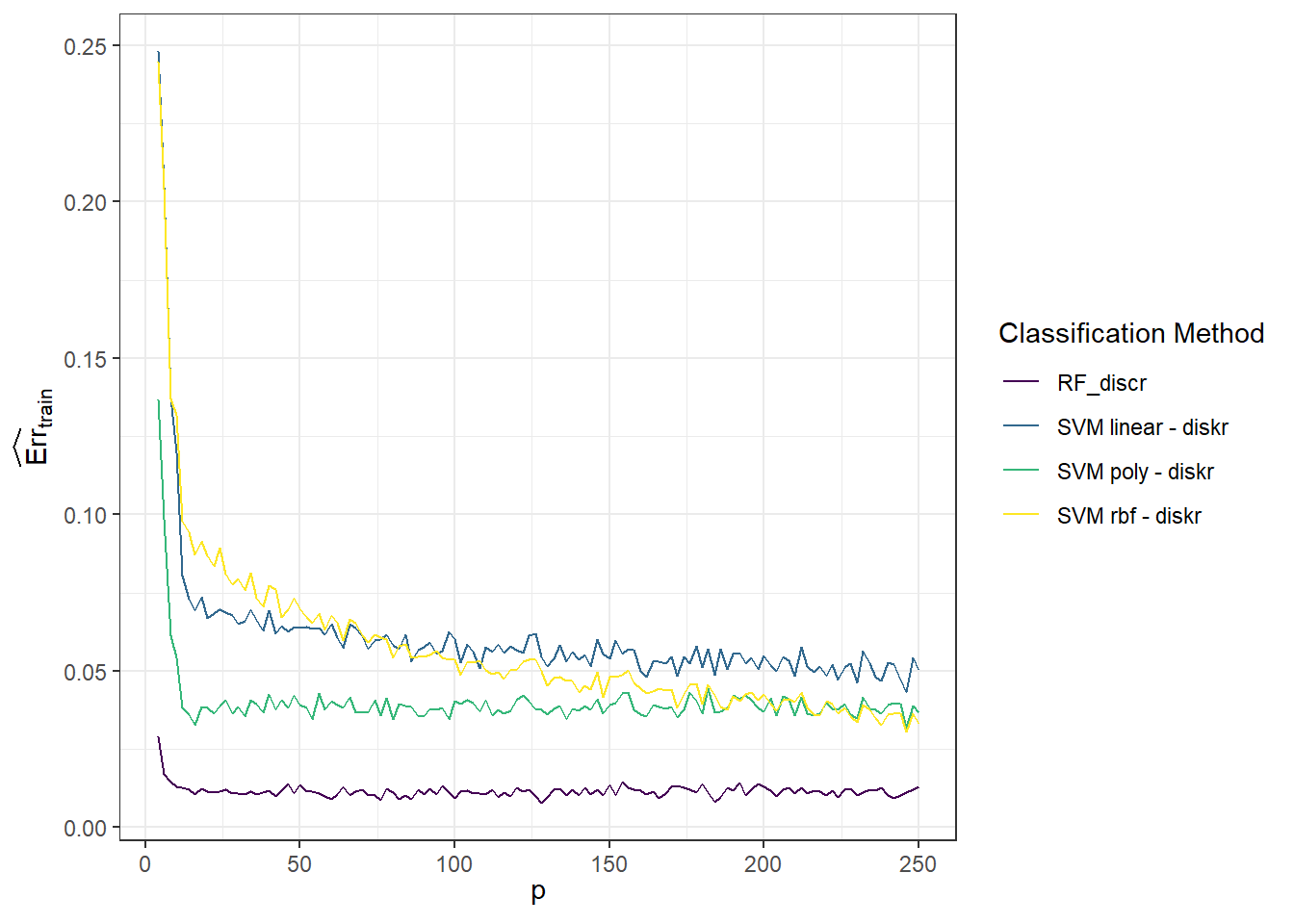

Figure 4.1: Graph of the dependence of training error rates for individual classification methods on the value of the parameter $p$.

Next, we’ll look at the test error rates, which is the graph we are most interested in.

Code

# for test data
SIMUL_params[, 2, ] |> 
  as.data.frame() |> 
  mutate(method = methods) |>
  pivot_longer(cols = as.character(p_vector), 
               names_to = 'p', 
               values_to = 'Err') |>
  mutate(method = factor(method, levels = methods, labels = methods, ordered = TRUE), 
         p = as.numeric(p)) |> 
  filter(method %in% c("RF_discr", "SVM linear - diskr",
                       "SVM poly - diskr", "SVM rbf - diskr")) |>
  ggplot(aes(x = p, y = Err, colour = method)) + 
  geom_line() + 
  theme_bw() + 
  labs(x = expression(p),
       y = expression(widehat(Err)[test]),
       colour = 'Classification Method') + 
  theme(legend.position = 'right')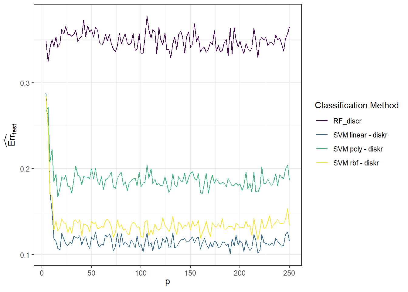

Figure 1.12: Graph of the dependence of test error rates for individual classification methods on the value of the parameter $p$.

Finally, let’s plot the graph for the time complexity of the methods.

Code

SIMUL_params[, 5, ] |> 
  as.data.frame() |> 
  mutate(method = methods) |>
  pivot_longer(cols = as.character(p_vector), 
               names_to = 'p', 
               values_to = 'Duration') |>
  mutate(method = factor(method, levels = methods, labels = methods, ordered = TRUE), 
         p = as.numeric(p)) |> 
  filter(method %in% c("RF_discr", "SVM linear - diskr",
                       "SVM poly - diskr", "SVM rbf - diskr")) |>
  ggplot(aes(x = p, y = Duration, colour = method, linetype = method)) + 
  geom_line() + 
  theme_bw() + 
  labs(x = expression(p),
       y = "Duration [s]",
       colour = 'Classification Method',
       linetype = 'Classification Method') + 
  theme(legend.position = 'right') + 
  scale_y_log10() +
  scale_colour_manual(values = c('deepskyblue2', 'deepskyblue2', 'tomato',
                                 'tomato', 'tomato')) + 
  scale_linetype_manual(values = c('solid', 'dashed',
                                   'solid', 'dashed', 'dotted'))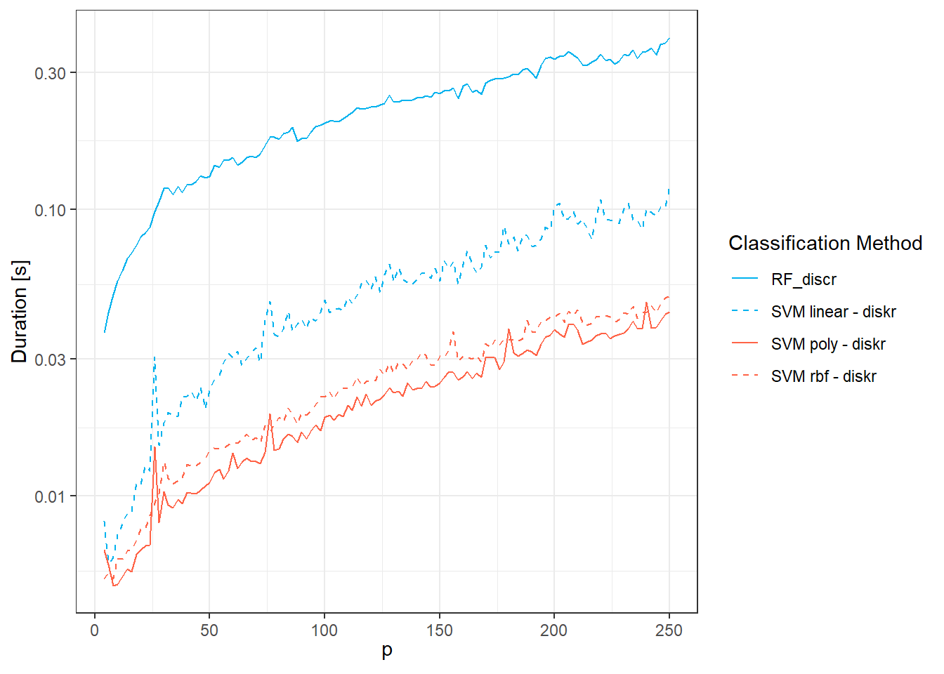

Figure 2.7: Graph of the dependence of the time complexity of methods for individual classification methods on the value of the parameter $p$.

Since the results are subject to random fluctuations and increasing the number of repetitions n.sim would be computationally intensive, let’s now smooth the curves of the average test error rates with respect to the parameter $p$.

Code

Dat <- SIMUL_params[, 2, ] |> 
  as.data.frame() |> t()

breaks <- p_vector
rangeval <- range(breaks)
norder <- 4
wtvec <- rep(1, 124)
# wtvec <- c(seq(50, 10, length = 4), seq(0.1, 0.1, length = 10), rep(1, 110))

bbasis <- create.bspline.basis(rangeval = rangeval, 
                               norder = norder, 
                               breaks = breaks)

curv.Lfd <- int2Lfd(2)

lambda.vect <- 10^seq(from = 3, to = 5, length.out = 50) # vector of lambda
gcv <- rep(NA, length = length(lambda.vect)) # empty vector for GCV storage

for(index in 1:length(lambda.vect)) {
  curv.Fdpar <- fdPar(bbasis, curv.Lfd, lambda.vect[index])
  BSmooth <- smooth.basis(breaks, Dat, curv.Fdpar, 
                          wtvec = wtvec) # smoothing
  gcv[index] <- mean(BSmooth$gcv) # average over all observed curves
}

GCV <- data.frame(
  lambda = round(log10(lambda.vect), 3),
  GCV = gcv
)

# find the minimum value
lambda.opt <- lambda.vect[which.min(gcv)]

curv.fdPar <- fdPar(bbasis, curv.Lfd, lambda.opt)
BSmooth <- smooth.basis(breaks, Dat, curv.fdPar,
                        wtvec = wtvec)
XXfd <- BSmooth$fd

fdobjSmootheval <- eval.fd(fdobj = XXfd, 
                           evalarg = seq(min(p_vector), max(p_vector), length = 101))

df_plot_smooth <- data.frame(
  method = rep(colnames(fdobjSmootheval), each = dim(fdobjSmootheval)[1]),
  value = c(fdobjSmootheval),
  p = rep(seq(min(p_vector), max(p_vector), length = 101), length(methods))
) |> 
  mutate(method = factor(method, levels = methods, labels = methods, ordered = TRUE))

Code

# for test data
p1 <- SIMUL_params[, 2, ] |> 
  as.data.frame() |> 
  mutate(method = methods) |>
  pivot_longer(cols = as.character(p_vector), 
               names_to = 'p', 
               values_to = 'Err') |>
  mutate(method = factor(method, levels = methods, labels = methods, ordered = TRUE), 
         p = as.numeric(p)) |> 
  filter(method %in% c("RF_discr", "SVM linear - diskr",
                       "SVM poly - diskr", "SVM rbf - diskr")) |>
  ggplot(aes(x = p, y = Err, colour = method, shape = method)) + 
  geom_point(alpha = 0.7, size = 0.6) + 
  theme_bw() + 
  labs(x = 'p',
       y = 'Test Error Rate',
       colour = 'Classification Method',
       linetype = 'Classification Method',
       shape = 'Classification Method') + 
  theme(legend.position = 'none',
        plot.margin = unit(c(0.1, 0.1, 0.3, 0.5), "cm"),
        panel.grid.minor.x = element_blank()) +
    # scale_y_log10() +
  geom_line(data = df_plot_smooth, aes(x = p, y = value, col = method,
                                       linetype = method),
            linewidth = 0.95) + 
  scale_colour_manual(values = c('deepskyblue2', 'deepskyblue2', #'tomato',
                                 'tomato', 'tomato'),
                      labels = methods_names) + 
  scale_linetype_manual(values = c('solid', 'dashed',
                                   'solid', 'dashed'#, 'dotted'
                                   ),
                        labels = methods_names) + 
  scale_shape_manual(values = c(16, 1, 16, 1),
                     labels = methods_names) +
  guides(colour = guide_legend(override.aes = list(size = 1.2, alpha = 0.7)),
         linetype = guide_legend(override.aes = list(linewidth = 0.8)))
p1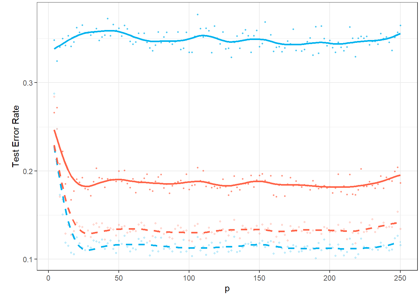

Figure 1.13: Graph of the dependence of test error rates for individual classification methods on the value of the parameter $p$.

Code

# ggsave("figures/kap6_sim_03diskr_curvesErr.tex", device = tikz, width = 4.5, height = 4.5)

Let’s add the computational time to the graph.

Code

Dat <- SIMUL_params[, 5, ] |> 
  as.data.frame() |> t()

breaks <- p_vector
rangeval <- range(breaks)
norder <- 4
wtvec <- rep(1, 124)
# wtvec <- c(seq(50, 10, length = 4), seq(0.1, 0.1, length = 10), rep(1, 110))

bbasis <- create.bspline.basis(rangeval = rangeval, 
                               norder = norder, 
                               breaks = breaks)

curv.Lfd <- int2Lfd(2)

lambda.vect <- 10^seq(from = 3, to = 5, length.out = 50) # vector of lambda
gcv <- rep(NA, length = length(lambda.vect)) # empty vector for GCV storage

for(index in 1:length(lambda.vect)) {
  curv.Fdpar <- fdPar(bbasis, curv.Lfd, lambda.vect[index])
  BSmooth <- smooth.basis(breaks, Dat, curv.Fdpar, 
                          wtvec = wtvec) # smoothing
  gcv[index] <- mean(BSmooth$gcv) # average over all observed curves
}

GCV <- data.frame(
  lambda = round(log10(lambda.vect), 3),
  GCV = gcv
)

# find the minimum value
lambda.opt <- lambda.vect[which.min(gcv)]

curv.fdPar <- fdPar(bbasis, curv.Lfd, lambda.opt)
BSmooth <- smooth.basis(breaks, Dat, curv.fdPar,
                        wtvec = wtvec)
XXfd <- BSmooth$fd

fdobjSmootheval <- eval.fd(fdobj = XXfd, 
                           evalarg = seq(min(p_vector), max(p_vector), length = 101))

df_plot_smooth_2 <- data.frame(
  method = rep(colnames(fdobjSmootheval), each = dim(fdobjSmootheval)[1]),
  value = c(fdobjSmootheval),
  p = rep(seq(min(p_vector), max(p_vector), length = 101), length(methods))
) |> 
  mutate(method = factor(method, levels = methods, labels = methods, ordered = TRUE))

Code

# for test data
p2 <- SIMUL_params[, 5, ] |> 
  as.data.frame() |> 
  mutate(method = methods) |>
  pivot_longer(cols = as.character(p_vector), 
               names_to = 'p', 
               values_to = 'Err') |>
  mutate(method = factor(method, levels = methods, labels = methods, ordered = TRUE), 
         p = as.numeric(p)) |> 
  filter(method %in% c("RF_discr", "SVM linear - diskr",
                       "SVM poly - diskr", "SVM rbf - diskr")) |>
  ggplot(aes(x = p, y = Err, colour = method, shape = method)) + 
  geom_point(alpha = 0.7, size = 0.6) + 
  theme_bw() + 
  labs(x = 'p',
       y = 'computational time',
       colour = 'Classification Method',
       linetype = 'Classification Method',
       shape = 'Classification Method') + 
  theme(legend.position = c(0.7, 0.16),#'right',
        plot.margin = unit(c(0.1, 0.1, 0.3, 0.5), "cm"),
        panel.grid.minor = element_blank(),
        legend.background = element_rect(fill='transparent'),
        legend.key = element_rect(colour = NA, fill = NA)) +
  scale_y_log10() +
  geom_line(data = df_plot_smooth_2, aes(x = p, y = value, col = method,
                                       linetype = method),
            linewidth = 0.95) + 
  scale_colour_manual(values = c('deepskyblue2', 'deepskyblue2', #'tomato',
                                 'tomato', 'tomato'),
                      labels = methods_names) + 
  scale_linetype_manual(values = c('solid', 'dashed',
                                   'solid', 'dashed'#, 'dotted'
                                   ),
                        labels = methods_names) + 
  scale_shape_manual(values = c(16, 1, 16, 1),
                     labels = methods_names) +
  guides(colour = guide_legend(override.aes = list(size = 1.2, alpha = 0.7)),
         linetype = guide_legend(override.aes = list(linewidth = 0.8)))
p2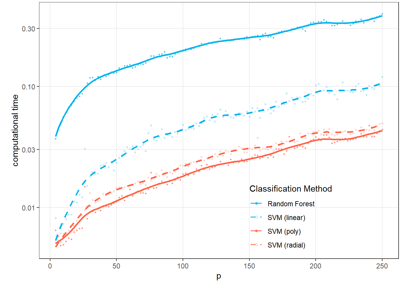

Figure 1.14: Graph of the dependence of computational time for individual classification methods on the value of the parameter $p$.

Code

# ggsave("figures/kap6_sim_03diskr_curvesTime.tex", device = tikz, width = 4.5, height = 4.5)

Detailed comments on the results of this simulation study can be found in the article.